Difference-in-Differences in Python

From the classic 2×2 design to staggered adoption and honest sensitivity

5.12classic 2×2 ATT · true effect 5.0

2.41Callaway–Sant’Anna · TWFE biased to 2.18

M = 15HonestDiD breakdown

Carlos Mendez

Nagoya University (GSID)

July 8, 2026

The Tension

Act I

An education ministry rolls out AI tutors in some cities — did it work, or were they already rising?

Some cities adopt AI tutoring bots; others do not. Scores climb in the treated cities.

But maybe those cities were already on the way up. How do you separate the policy from the trend it rode in on?

This is the core challenge of policy evaluation: separating the genuine effect of an intervention from pre-existing trends and selection differences between treated and untreated groups. Card and Krueger (1994) pioneered the answer with New Jersey vs Pennsylvania fast-food employment after a minimum-wage rise.

DiD uses the control group as a mirror for the treated group’s missing counterfactual

Both groups track in lockstep for periods 0–4, then the treated group jumps at treatment onset. The gap after period 5 is the effect.

Spoiler-style framing figure. Don’t dwell on the numbers yet — just plant the idea: if the two groups moved in parallel before treatment, the control group’s post-treatment path is what the treated group would have done absent the policy. The gap is the causal effect.

Where we’re going

• The logic: why differencing twice identifies the ATT under parallel trends
• The classic 2×2 estimator and a formal pre-trends test
• Event studies: the effect period by period
• Why naive TWFE breaks under staggered timing — and how Callaway–Sant’Anna fixes it
• HonestDiD: how wrong can parallel trends be before the answer flips?

The Investigation

Act II

DiD estimates the ATT — the effect on the units that actually got treated

\[\text{ATT} = E[Y^1_k - Y^0_k \mid \text{Post}]\]

The average gap between what treated units experienced and what they would have experienced without the policy.

\(E[Y^0_k\mid\text{Post}]\) — the treated group’s untreated outcome — is a counterfactual we never observe. DiD reconstructs it from the control group.

The fundamental problem of causal inference: for any one unit we see only one potential outcome. We give up on individual effects and target the average over the treated subpopulation. ATT, not ATE — this is the policy-relevant quantity: did it help the people it was aimed at?

Difference twice: kill the level gap, then kill the common trend

\[\hat{\delta}^{2 \times 2}_{kU} = \big( \bar{Y}_k^{Post} - \bar{Y}_k^{Pre} \big) - \big( \bar{Y}_U^{Post} - \bar{Y}_U^{Pre} \big)\]

The first difference removes time-invariant differences between groups; the second removes the trend common to both.

Algebra splits this into \(\underbrace{\text{ATT}}\) plus a \(\underbrace{\text{non-parallel-trends bias}}\). The bias vanishes exactly when parallel trends holds.

The Cunningham (2021) decomposition: the 2×2 estimator equals the ATT plus a bias term comparing the untreated trajectories of the two groups. If their untreated outcomes would have moved in parallel, the bias is zero and DiD cleanly identifies the ATT.

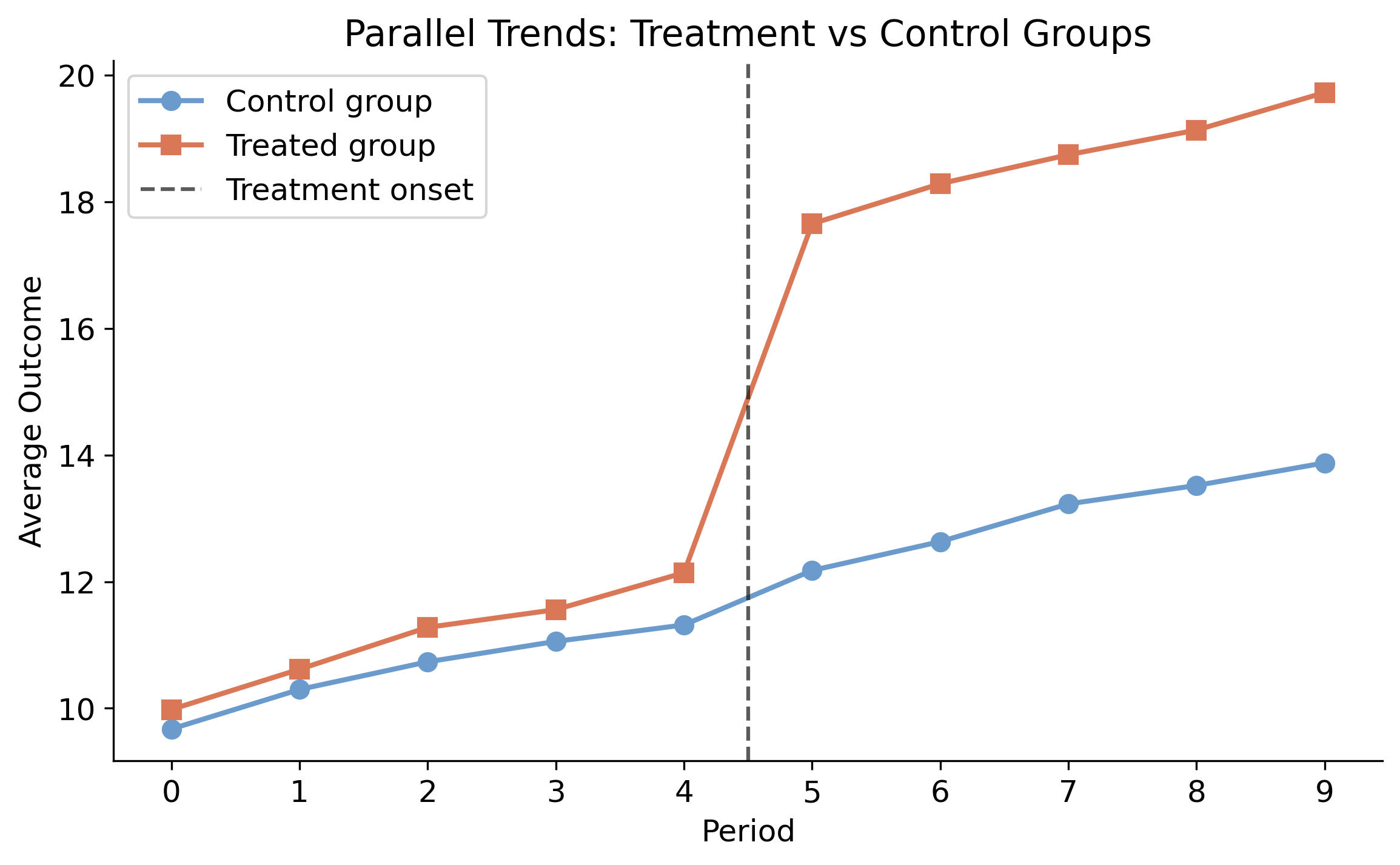
Parallel trends is about slopes, not levels — and it is fundamentally untestable

\[E[Y^0_k|\text{Post}] - E[Y^0_k|\text{Pre}] = E[Y^0_U|\text{Post}] - E[Y^0_U|\text{Pre}]\]

Two cities can sit at different score levels; DiD only needs them to have been rising at the same speed absent treatment.

We can check pre-treatment trends, but never the post-treatment counterfactual — which is why Act III brings sensitivity analysis.

This is the load-bearing assumption. It does not require equal levels — only equal trends. And the post-treatment half is untestable because the treated group’s untreated outcome is never observed. Roth (2022) also warns that conditioning on passing a pre-test distorts later inference.

The lab: a 100-unit, 10-period panel built with a known true effect of 5.0

• 1,000 observations — 100 units × 10 periods (0–9)
• 50 treated, 50 control; treatment switches on at period 5
• True effect = 5.0 baked in, so every estimate has a ground truth to hit

A built-in true_effect column gives every estimate a known target to hit.

Using simulated data with a known effect is the pedagogical move: we can verify the estimator recovers the truth before trusting it on real data where the truth is unknown. The 2×2 crosstab is perfectly balanced — 250 observations in each of the four cells.

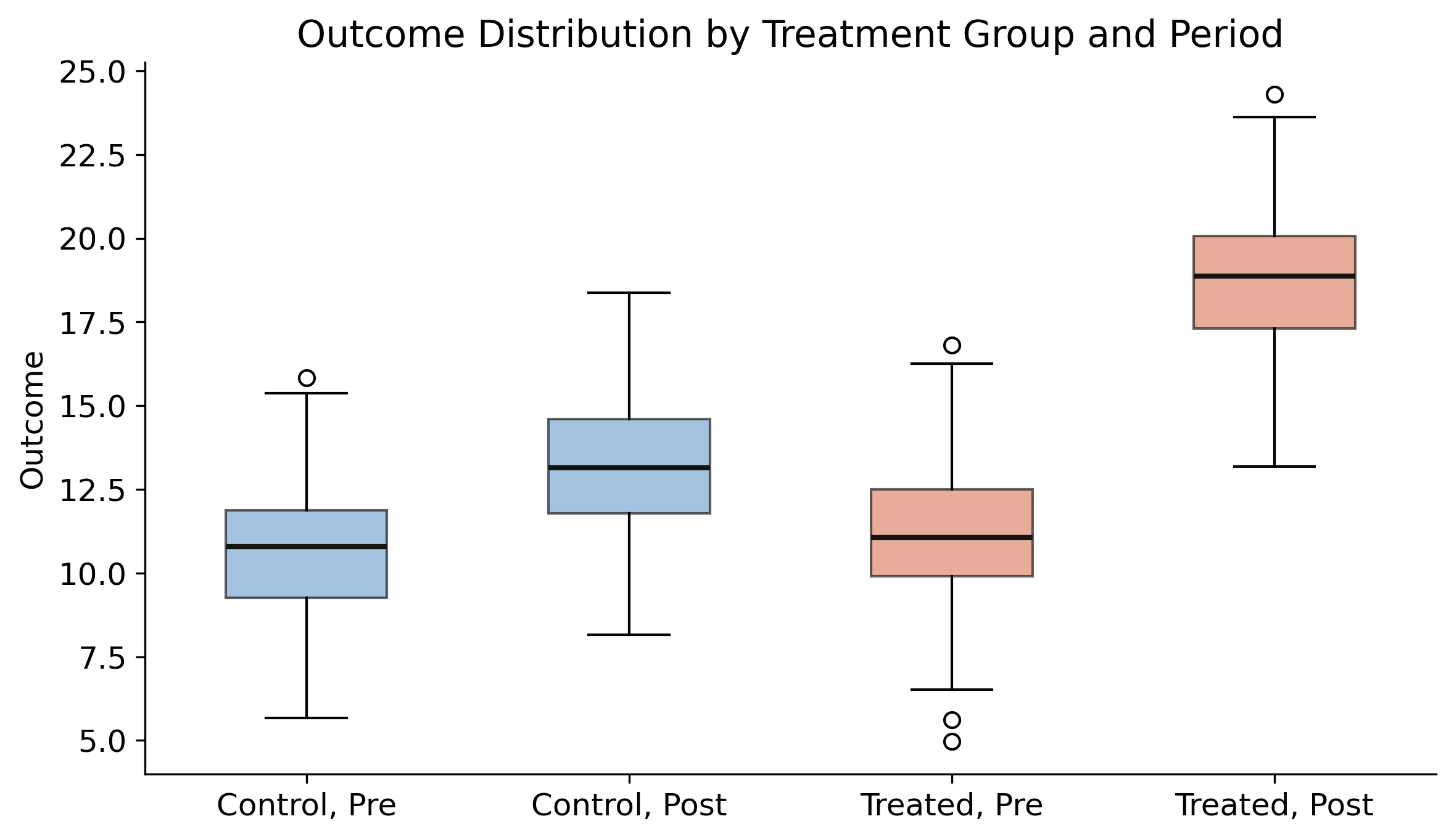
Before treatment the two groups overlap; after, the treated box jumps far higher

Outcome distributions by group × period. Control (steel) and treated (orange) overlap pre-treatment near 10.6–11.1; the treated box jumps to ~18.9 post-treatment.

The raw means already tell the story: pre-treatment the control mean is 10.61 and treated 11.11 — a negligible 0.50 gap. Post-treatment the control rises to 13.09 (+2.47) but the treated jumps to 18.71 (+7.59). The extra gain, 7.59 − 2.47 = 5.12, is the DiD estimate before we run any regression.

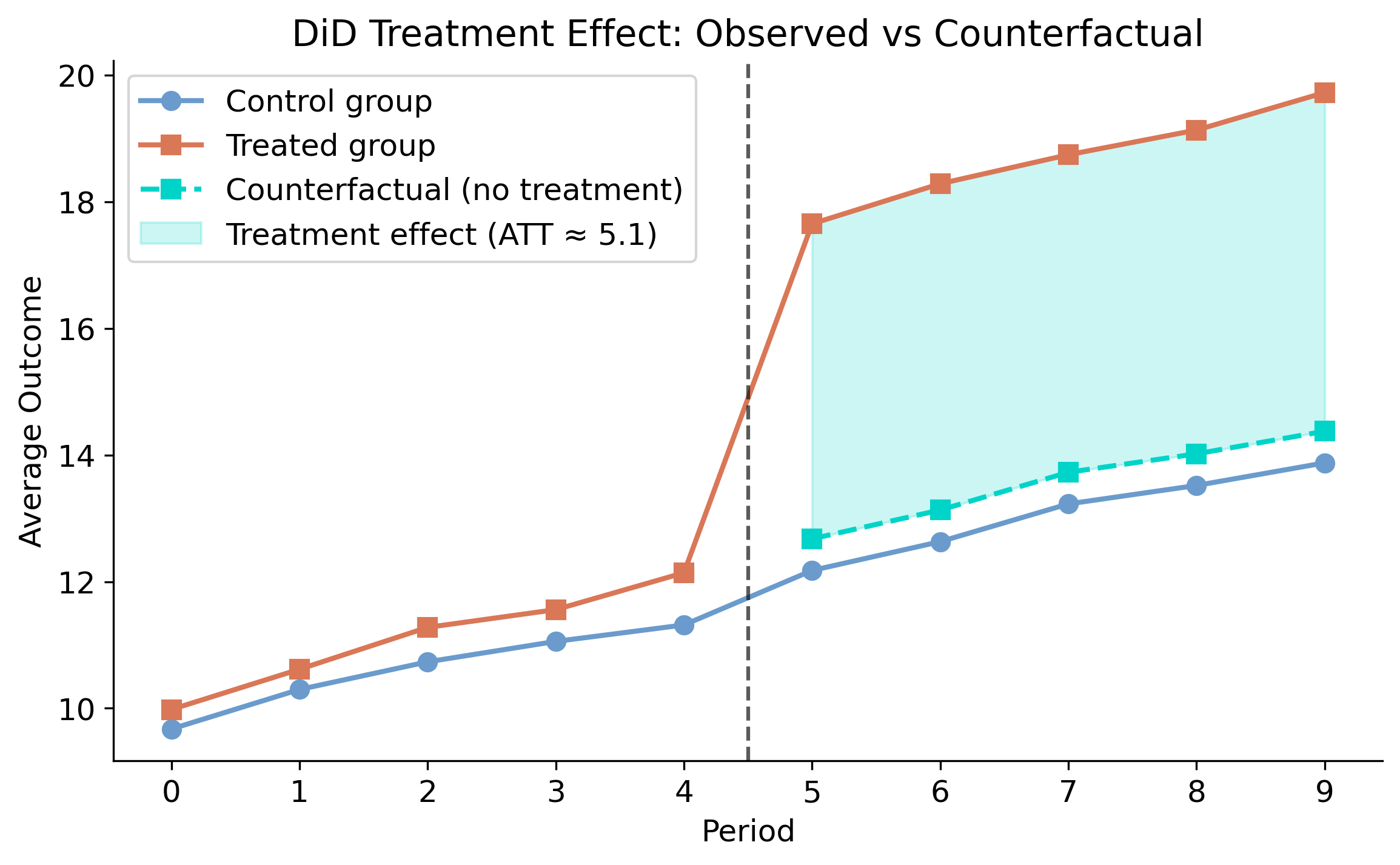
The shaded gap is the causal effect: treated outcomes minus their projected counterfactual

The teal dashed line is the control group’s path shifted to the treated group’s pre-level — the no-treatment counterfactual. The shaded gap is the ~5.1 ATT.

This makes the DiD logic tangible. We build the counterfactual by shifting the control group’s post-treatment trajectory up by the pre-treatment level gap between the groups. The shaded area between the actual treated outcomes and that counterfactual is the estimated causal effect — about 5.1 per period. The control group is the mirror.

Six lines fit the classic 2×2 estimator with the diff-diff package

from diff_diff import DifferenceInDifferences, generate_did_data
data = generate_did_data(n_units=100, n_periods=10,
                         treatment_effect=5.0, treatment_period=5, seed=42)
did = DifferenceInDifferences()
res = did.fit(data, outcome="outcome", treatment="treated", time="post")
res.print_summary()   # ATT = 5.1216, 95% CI [4.6399, 5.6034]

A scikit-learn-style API: build the estimator, call .fit() with the column names for outcome, treatment, and the pre/post time indicator. The diff-diff package validates 13+ DiD estimators against their R counterparts. Full script is in the post.

The classic estimator recovers 5.12 — within 2.4% of the true 5.0

5.12

Classic 2×2 \(\widehat{\text{ATT}}\) (SE 0.25, \(t = 20.9\)) · 95% CI [4.64, 5.60] covers the true 5.0

The 95% confidence interval [4.64, 5.60] comfortably contains the true value of 5.0. The 0.12 overshoot is sampling variability, not bias. With one treatment time and two groups, the classic estimator is exactly right for the job.

A formal pre-trends test fails to reject parallel trends: slope gap 0.12, p = 0.29

Group	Pre-trend slope	SE
Treated	0.5262	0.0839
Control	0.4047	0.0798
Difference	0.1216	0.1158

\(t = 1.05\), \(p = 0.29\) — fail to reject equal slopes. But failing to reject is not confirming: the test has low power with only 5 pre-periods.

The treated and control slopes differ by just 0.12, far from significant. This removes the most obvious objection to parallel trends but cannot prove it. With only 5 pre-treatment periods the test has limited power, and Roth (2022) shows pre-testing can distort later inference. That is precisely why HonestDiD enters in Act III.

The event study splits the single ATT into one effect per period relative to treatment

\[Y_{it} = \gamma_i + \lambda_t + \sum_{k=-K+1}^{-2}\beta_k^{lead}D_{it}^k + \sum_{k=0}^{L}\beta_k^{lag}D_{it}^k + \varepsilon_{it}\]

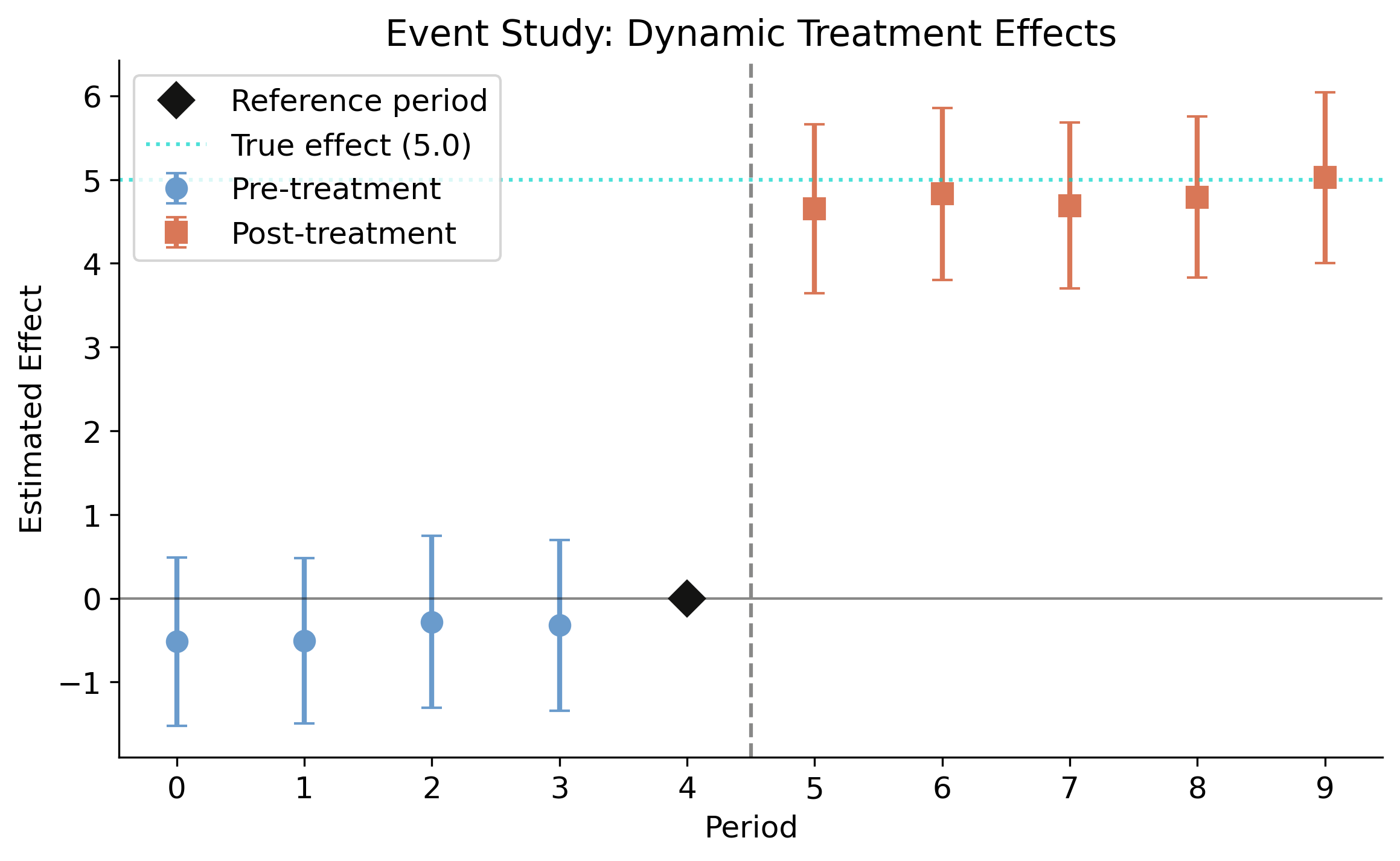
The leads \(\beta_k^{lead}\) are placebo tests (should be ~0); the lags \(\beta_k^{lag}\) trace how the effect evolves. The period before treatment is the omitted reference.

This one equation does two jobs at once: the leads test parallel trends period by period, and the lags reveal whether the effect appears instantly, builds up, or fades. Unit and time fixed effects implement the “two-way” structure. Period k = −1 is normalized to zero as the baseline.

Leads sit on zero, lags snap to ~5.0 — the visual signature of a clean DiD

Pre-treatment coefficients (steel) hover at zero with CIs crossing it; post-treatment coefficients (orange) jump to ~5.0, matching the teal true-effect line.

Pre-treatment leads range from −0.52 to −0.28, all insignificant (p > 0.3) — the placebo test passes. Post-treatment lags run 4.65 to 5.02, all with t > 9. The effect is stable: no build-up, no fade-out. The teal dotted line at 5.0 shows every post estimate landing on the truth.

Real policies roll out city by city — and that staggered timing breaks naive TWFE

• 3,000 observations — 300 units × 10 periods
• Three cohorts adopt at periods 3, 5, 7 (60, 75, 75 units)
• 90 never-treated units — a clean control group
• Effects grow over time by construction (2.0 → 3.2 for the earliest cohort)

TWFE fits one pooled \(\delta\) — a weighted average of many 2×2 comparisons, some of them poisoned.

The TWFE specification is Y_it = γ_i + λ_t + δ·D_it + ε_it. With a single treatment time, δ is correct. With staggered timing it becomes a weighted average of all pairwise 2×2 comparisons — and some of those use already-treated units as controls. When effects grow over time, that drags the estimate down.

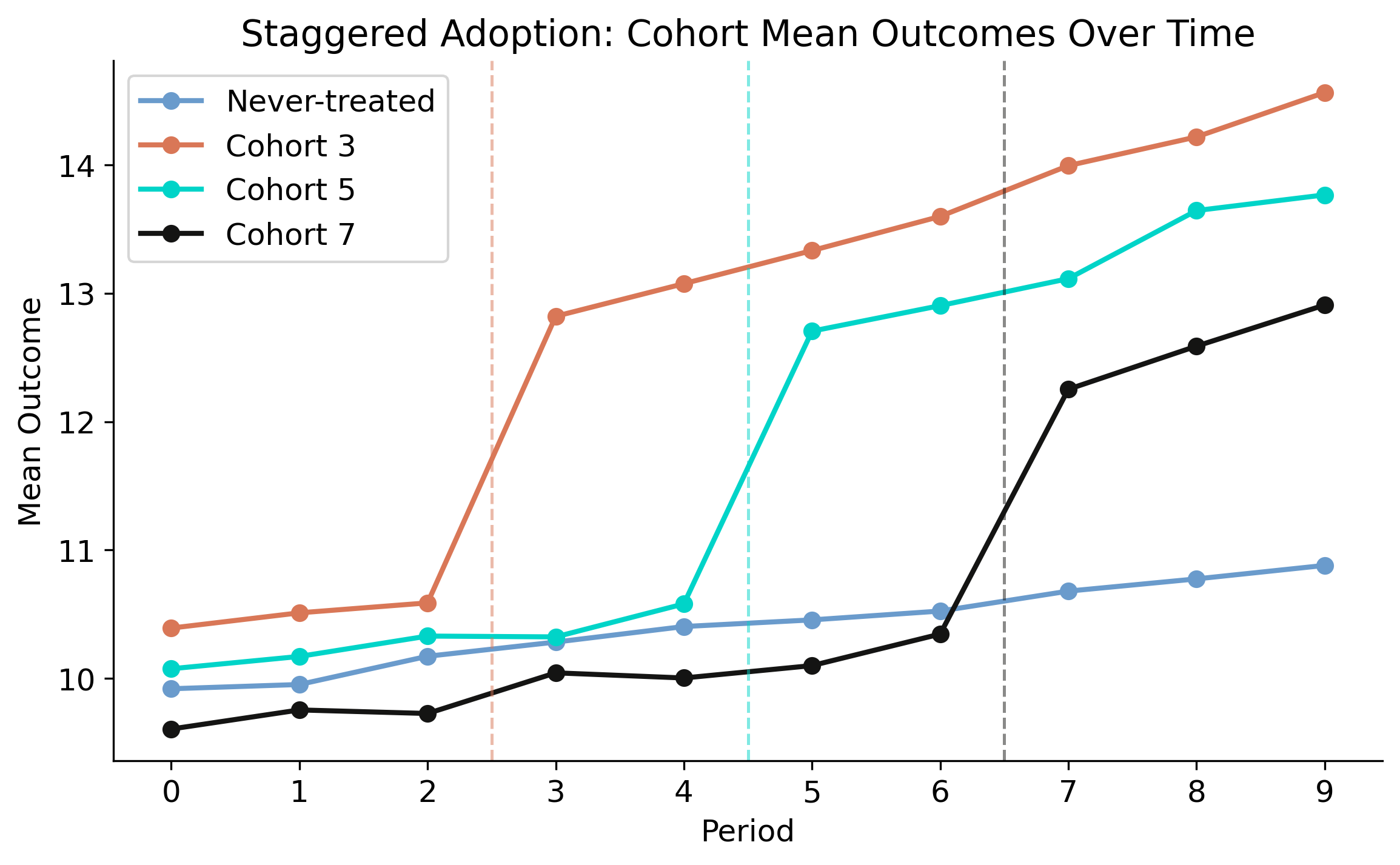
Cohorts move in parallel, then jump at their own onset — TWFE then mis-uses early adopters as controls

Four cohorts track together pre-treatment, then cohort 3 (orange), 5 (teal), 7 (near black) each jump at its onset; never-treated (steel) drifts gently up.

Between periods 3 and 7, TWFE uses cohort 3 — already treated and elevated — as a comparison for the not-yet-treated cohort 7. Cohort 3’s outcomes already carry a treatment effect of ~2.8, so the comparison understates cohort 7’s true effect. This is the forbidden comparison made visible.

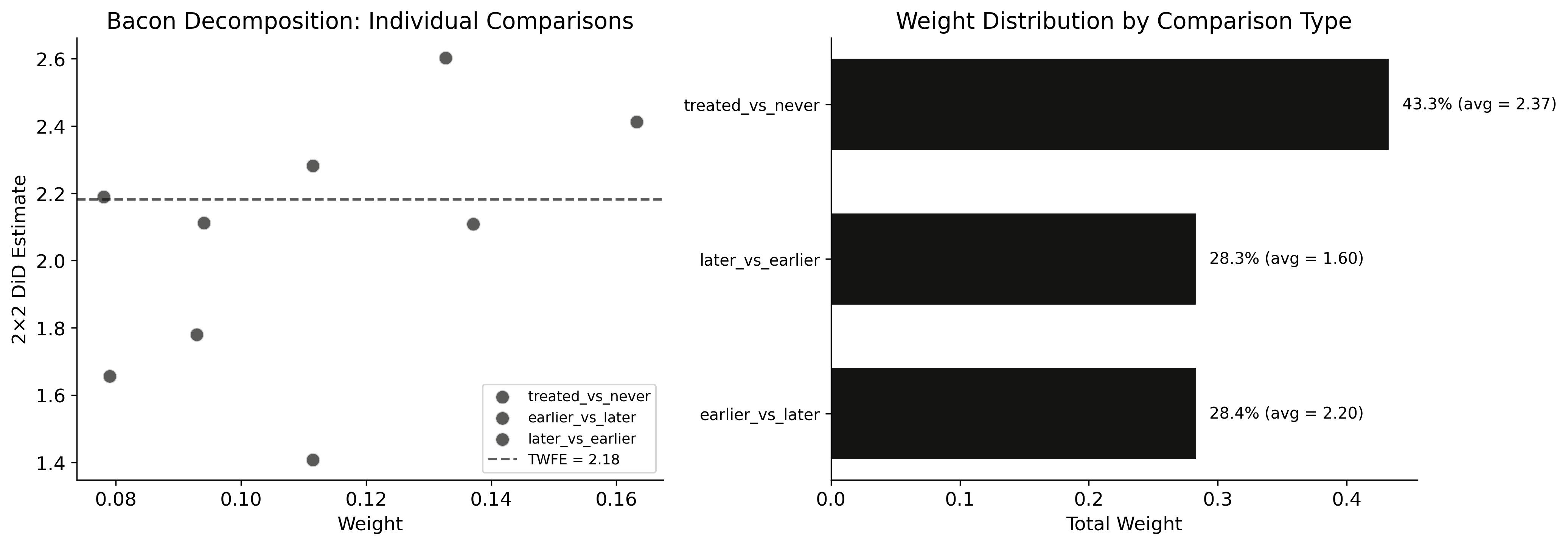
The Goodman–Bacon decomposition shows 28.3% of TWFE’s weight is on forbidden comparisons

Left: each 2×2 comparison as a point, forbidden ones (dark orange) cluster low. Right: weight by type — nearly a third on forbidden comparisons.

Comparison type	Weight	Avg effect
Treated vs never-treated (clean)	0.433	2.37
Earlier vs later treated	0.284	2.20
Later vs earlier (forbidden)	0.283	1.60

The decomposition writes TWFE as a weighted average of every 2×2. The forbidden comparisons — already-treated units as controls — carry 28.3% of the weight and an average of only 1.60, well below the 2.37 from clean comparisons. That downward pull is what biases TWFE.

Forbidden comparisons drag TWFE down to a biased 2.18

2.18

Naive TWFE \(\hat{\delta}\) · downward-biased by 28.3% weight on forbidden comparisons (avg effect 1.60)

For a policymaker reading the TWFE number, 2.18 understates the true impact. The contamination is not a rounding error — it is a structural feature of pooling heterogeneous, dynamically-growing effects with already-treated controls.

Callaway–Sant’Anna rebuilds the estimate from clean group-time ATTs only

\[\text{ATT}(g,t) = E[Y_t - Y_{g-1}\mid G=g] - E[Y_t - Y_{g-1}\mid G=\infty]\]

Each building block is a 2×2 that compares cohort \(g\) against the never-treated group only — every forbidden comparison eliminated by construction.

A doubly robust version reweights controls (propensity) and models their outcome change (regression): valid if either is right.

CS computes a separate ATT for each cohort g and calendar period t, using only never-treated controls, then aggregates with valid weights. The doubly robust estimator is belt-and-suspenders: inverse-probability weighting plus outcome regression, consistent if either model is correctly specified.

Theory vs naive: same data, but CS uses only valid comparisons

Naive TWFE

• one pooled coefficient
• 28.3% weight on forbidden comparisons
• \(\hat{\delta} = 2.18\) (biased low)
• hides the dynamics

Callaway–Sant’Anna

• clean group-time ATTs
• never-treated controls only
• overall \(\widehat{\text{ATT}} = 2.41\)
• recovers the growth path

Same staggered data, two estimators. CS’s 2.41 is a 10% upward correction over TWFE’s 2.18 — precisely the bias the Bacon decomposition predicted. And CS does something TWFE cannot: it preserves the period-by-period dynamics instead of collapsing them into one number.

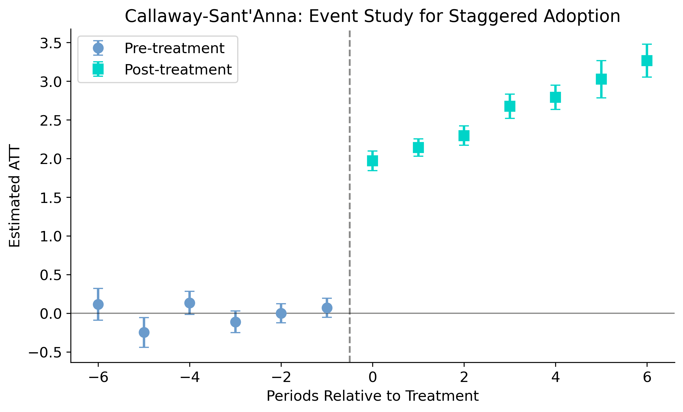
CS recovers a clean 2.41, and the effect grows from 1.97 to 3.27 over six periods

CS event study: pre-treatment effects pinned near zero (period −1 = 0 by construction); post-treatment effects rise steadily from ~2.0 to ~3.3.

Overall CS ATT = 2.41 (SE 0.06, p < 0.001), CI [2.31, 2.52] — above TWFE’s 2.18, confirming the downward bias. The seven pre-treatment coefficients all hover near zero (none individually significant), and the lags climb from 1.97 immediately post-treatment to 3.27 by six periods out. The growing path is exactly the case where TWFE fails worst.

Does machine-selecting comparisons make this causal? No — parallel trends still carries the weight

Objection. Switching from TWFE to Callaway–Sant’Anna can’t manufacture identification.

Response. Correct. CS only removes contaminated comparisons; the ATT is still identified only under parallel trends and no anticipation. It buys credibility on the timing problem, not on the untestable counterfactual — so we stress-test that next.

Steelman, don’t strawman. CS fixes the aggregation problem (forbidden comparisons), not the identifying assumption. Parallel trends in the post-treatment period remains untestable. That honest gap is what HonestDiD is built to quantify.

The Resolution

Act III

HonestDiD asks: how big a parallel-trends violation before the answer flips?

\[|\delta_t| \leq M \cdot \max_{t' < g}|\delta_{t'}|, \quad \text{for all } t \geq g\]

\(M\) is a stress dial: \(M=0\) assumes perfect parallel trends; \(M=5\) allows post-treatment violations five times the worst pre-treatment one. The breakdown value is where the CI first touches zero.

Rambachan & Roth (2023) replace the all-or-nothing parallel-trends assumption with a bounded one. As M rises, the robust CI widens. The breakdown value of M — where significance is lost — is the single most informative robustness number you can report.

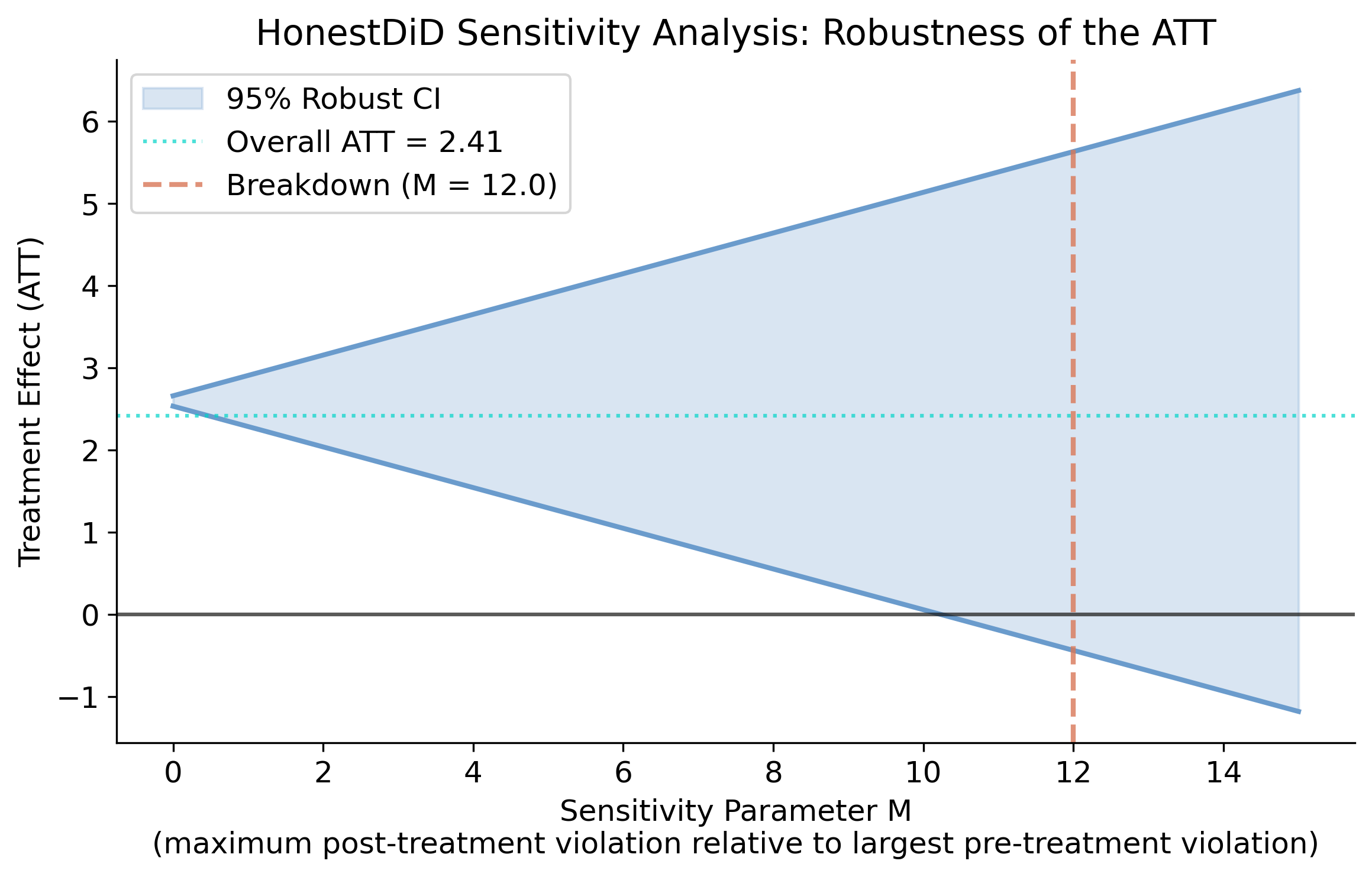
The CI stays above zero even when violations are 15× the worst pre-trend

Robust 95% CI (steel band) widening with M; ATT (teal) flat at 2.41; the lower bound is still positive (0.38) at the M = 15 grid edge (orange line).

At \(M=0\): CI [2.53, 2.66]. At \(M=15\): CI [0.38, 4.81] — still excludes zero.

The band expands symmetrically as M grows. At M = 10 the lower bound is still 1.10; at M = 15 it is 0.38 — the grid edge, with the true breakdown lying even further out. In applied work a breakdown above M = 3 is considered strong. This result clears that bar five times over.

The conclusion survives violations 15× worse than anything seen pre-treatment

M = 15

HonestDiD breakdown value · CI excludes zero even at 15× the largest pre-treatment deviation

To overturn the effect, post-treatment parallel-trend violations would have to exceed 15 times the worst pre-treatment departure — an extreme structural break coinciding exactly with treatment timing. Even a determined skeptic would struggle to argue the treatment did nothing.

Three estimators, one honest verdict: the effect is real, growing, and robust

Setting	Estimator	\(\widehat{\text{ATT}}\)
Single timing	Classic 2×2	5.12
Staggered (naive)	TWFE	2.18
Staggered (clean)	Callaway–Sant’Anna	2.41

Always report the breakdown value alongside the estimate — here \(M = 15\), exceptionally robust.

The classic estimator nails 5.0 when timing is uniform. Under staggered timing, naive TWFE is biased to 2.18; CS corrects it to 2.41 and reveals the growth dynamics; HonestDiD certifies robustness at M = 15. Caveats: synthetic data, linearly-growing effects, no spillovers — real applications need covariates and additional robustness checks.

Let the design — not the default regression — choose your comparisons.

The single takeaway. Under staggered timing, the default TWFE coefficient silently mixes forbidden comparisons; a modern estimator that uses only clean comparisons, paired with an honest sensitivity bound, is the difference between a biased 2.18 and a credible, robust 2.41.