Covariates in Difference-in-Differences

The LaLonde test in Python — when do covariates rescue a DiD?

3,621naive DiD · 2× too large

1,711–1,993covariates in the trend

1,794experimental benchmark (ATT)

Carlos Mendez

Nagoya University (GSID)

July 17, 2026

The Puzzle

Act I

The same job-training program, two very different answers

A program trained disadvantaged workers. A randomized trial found it raised earnings by about $1,794.

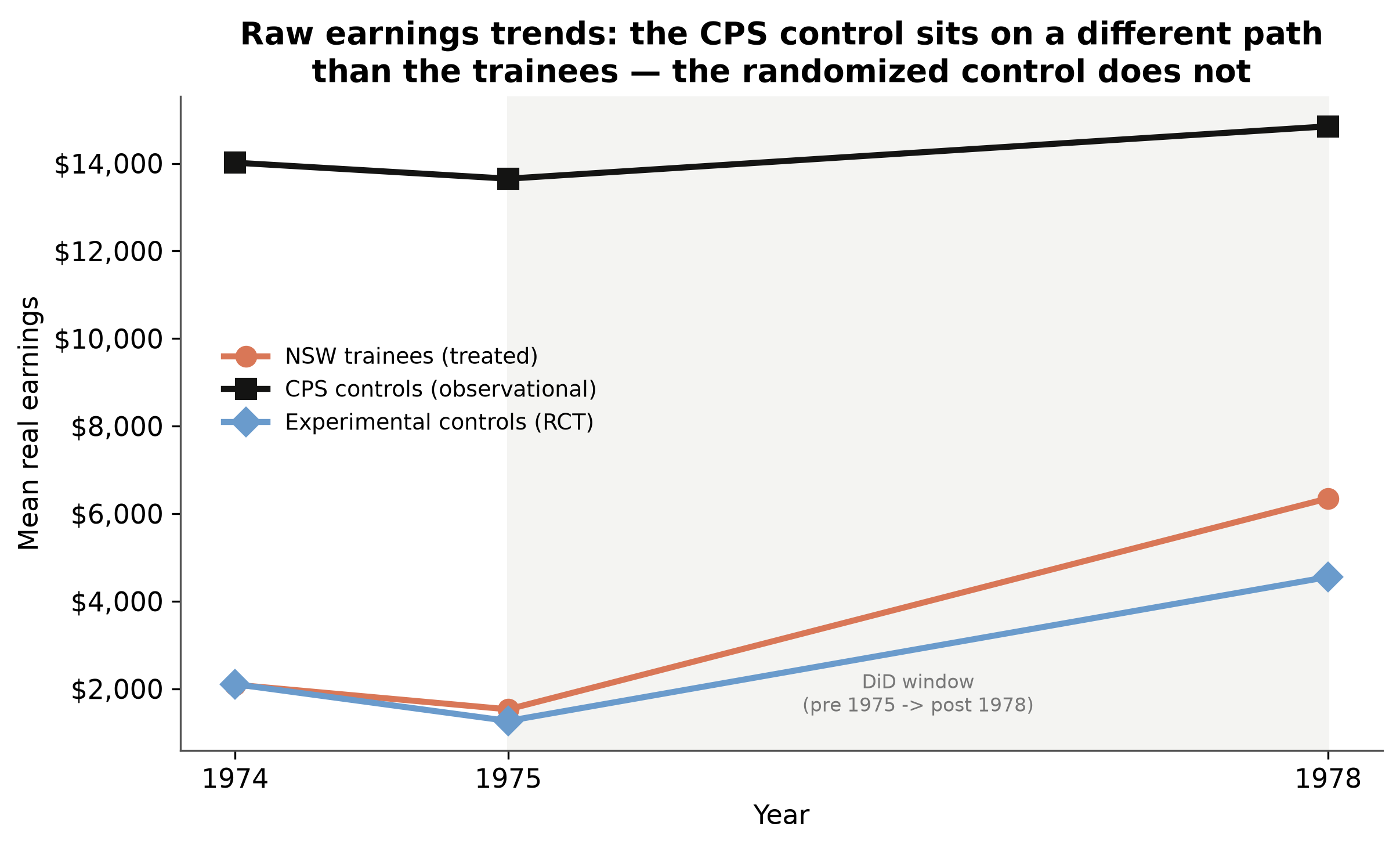
Throw away the randomized control group, swap in a survey of ordinary Americans, and run the usual difference-in-differences with covariates. Do you still recover $1,794?

Robert LaLonde asked exactly this in 1986 — and launched the credibility revolution when the answer was “no.”

The hook: we KNOW the answer because an RCT exists. The question is whether an observational estimator can find it, and whether the way we use covariates matters.

The setup

Following Scott Cunningham’s Mixtape Substack, we reproduce the test in Python.

• Data: Dehejia-Wahba subsample — 185 NSW trainees + 15,992 CPS controls.
• Panel: two periods, pre = 1975, post = 1978. Outcome = real earnings.
• Estimand: the ATT (effect on the treated). Design: observational.
• Ground truth: the experimental ATT ≈ $1,794.

Tip

Swapping the experimental control for CPS changes the ATE, but the treated group stays — so the ATT target is unchanged at $1,794.

Why the naive DiD fails: covariate imbalance

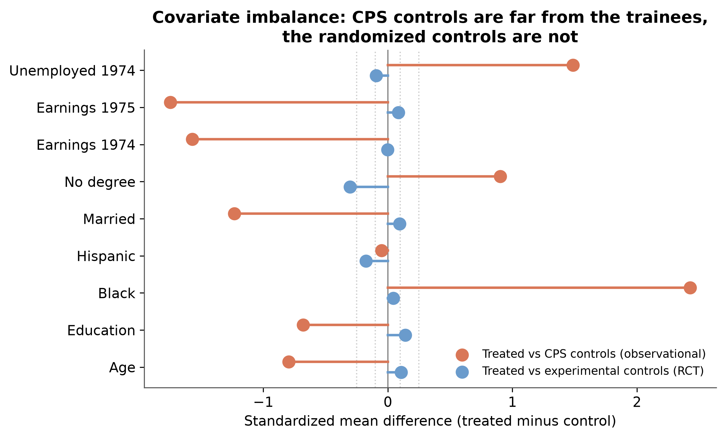
CPS controls differ from trainees by +2.3 SD on race and −1.6 SD on prior earnings. The randomized controls do not.

Different groups, different trends

The CPS control sits on a different level and slope. Assuming the trainees would have followed it is not credible — this is where covariates must work.

Four regressions, one number

The 2×2 DiD ATT is computed identically by:

1. Saturated dummies (treatment × post interaction)
2. Two-way fixed effects + post × treatment
3. First-difference regression on treatment
4. Across-group regression on post

We use the saturated form — it is the one that lets us add time-invariant covariates in different places and watch what happens.

The Spec Ladder

Act II — where does the covariate enter?

Three ways to add a covariate

A covariate \(X\) can enter a DiD in three fundamentally different places:

Placement	Formula	What it changes
Level	\(+ X\)	the intercept (additive control)
Effect	\(X \times D\)	the treatment effect (heterogeneity)
Trend	\(X \times \text{post}\)	the counterfactual trend

Only the last one addresses why the naive estimate is wrong. Watch the estimate as we climb the ladder.

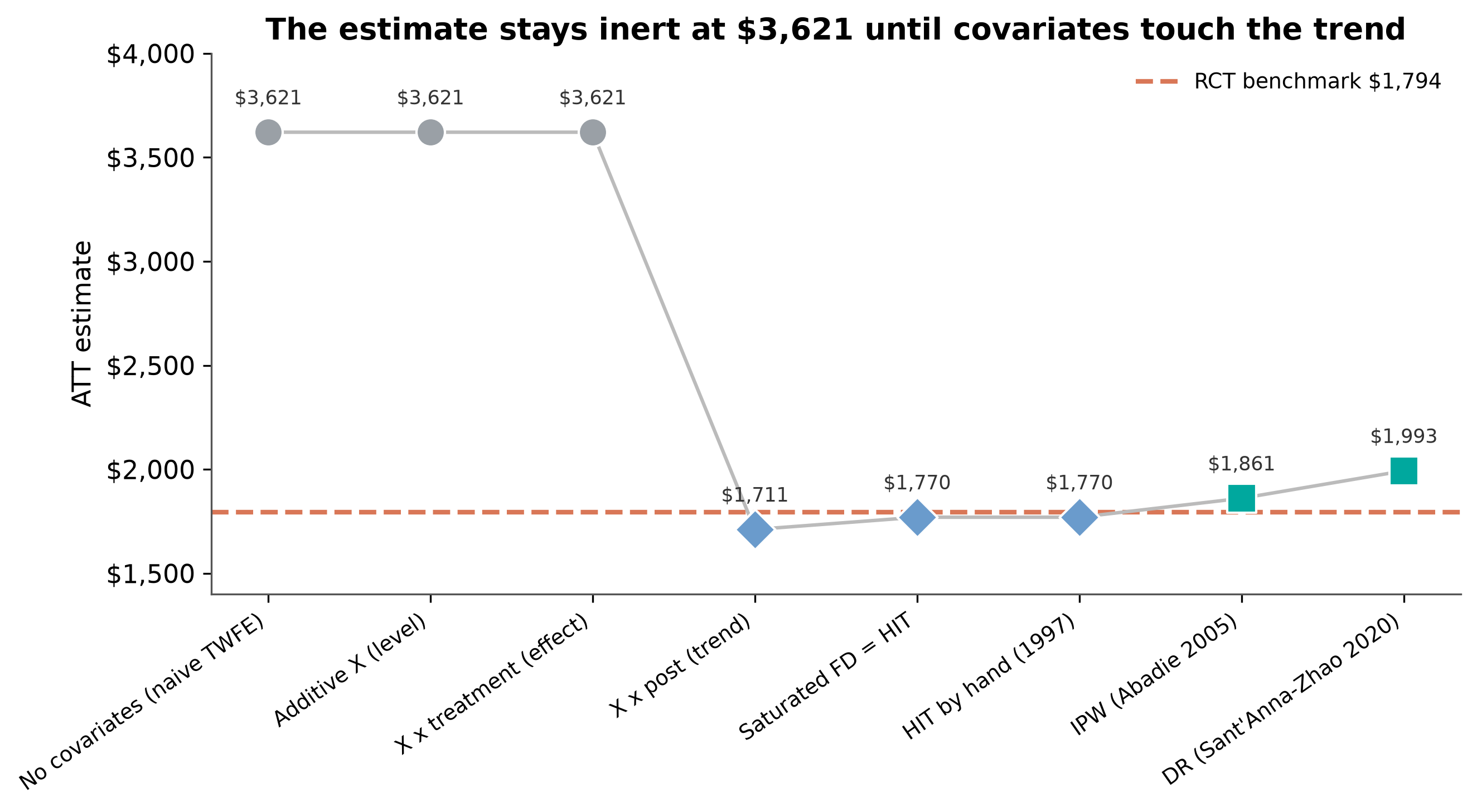
The estimate stays inert…

• Spec 0 — No covariates → $3,621

• Spec A — Additive \(X\) (level) → $3,621 · inert

• Spec BT — \(X \times\) treatment (effect) → $3,621 · inert

Time-invariant covariates in the level or the effect never touch the control’s trend. Nothing moves.

…until covariates touch the trend

• Spec B — \(X \times \text{post}\) (trend) → $1,711 ✅

• Spec C — saturated first differences = HIT (1997) → $1,770 ✅

• IPW (Abadie 2005) → $1,861 · DR (Sant’Anna-Zhao 2020) → $1,993

The instant covariates bend the counterfactual trend, the estimate snaps to the benchmark.

The cliff

The decision rule

flowchart LR
    Q{"Where does X enter?"}
    Q -->|level / effect| I["inert · ~3,621"]
    Q -->|trend / propensity| C["corrected · ~1,794"]
    C -.recovers.-> B["RCT benchmark 1,794"]

Covariates in DiD are not a robustness knob — they perform a function: satisfying conditional parallel trends and relaxing constant treatment effects.

The Payoff

Act III

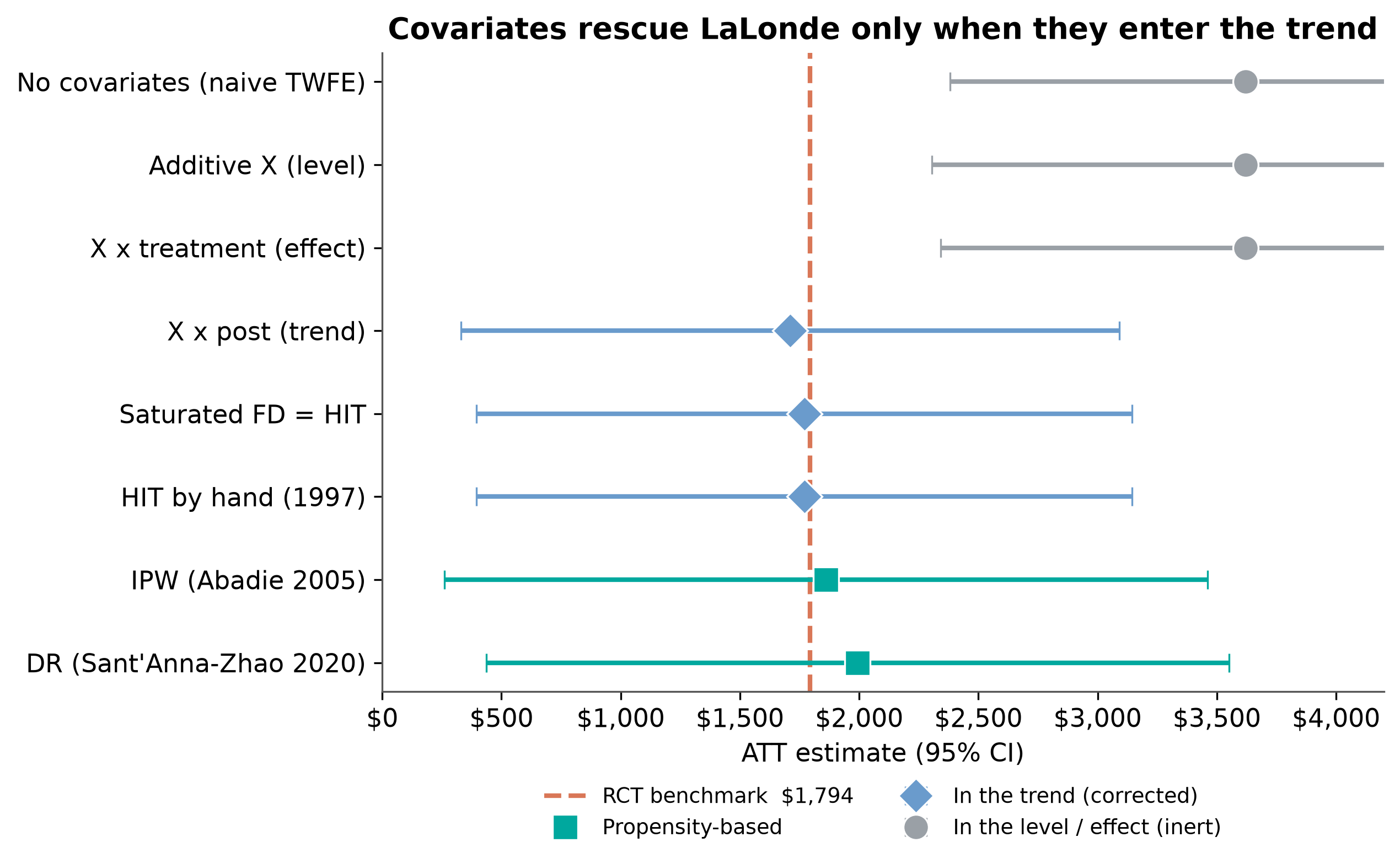
Covariates rescue LaLonde only when they enter the trend

Independent check: the diff-diff package

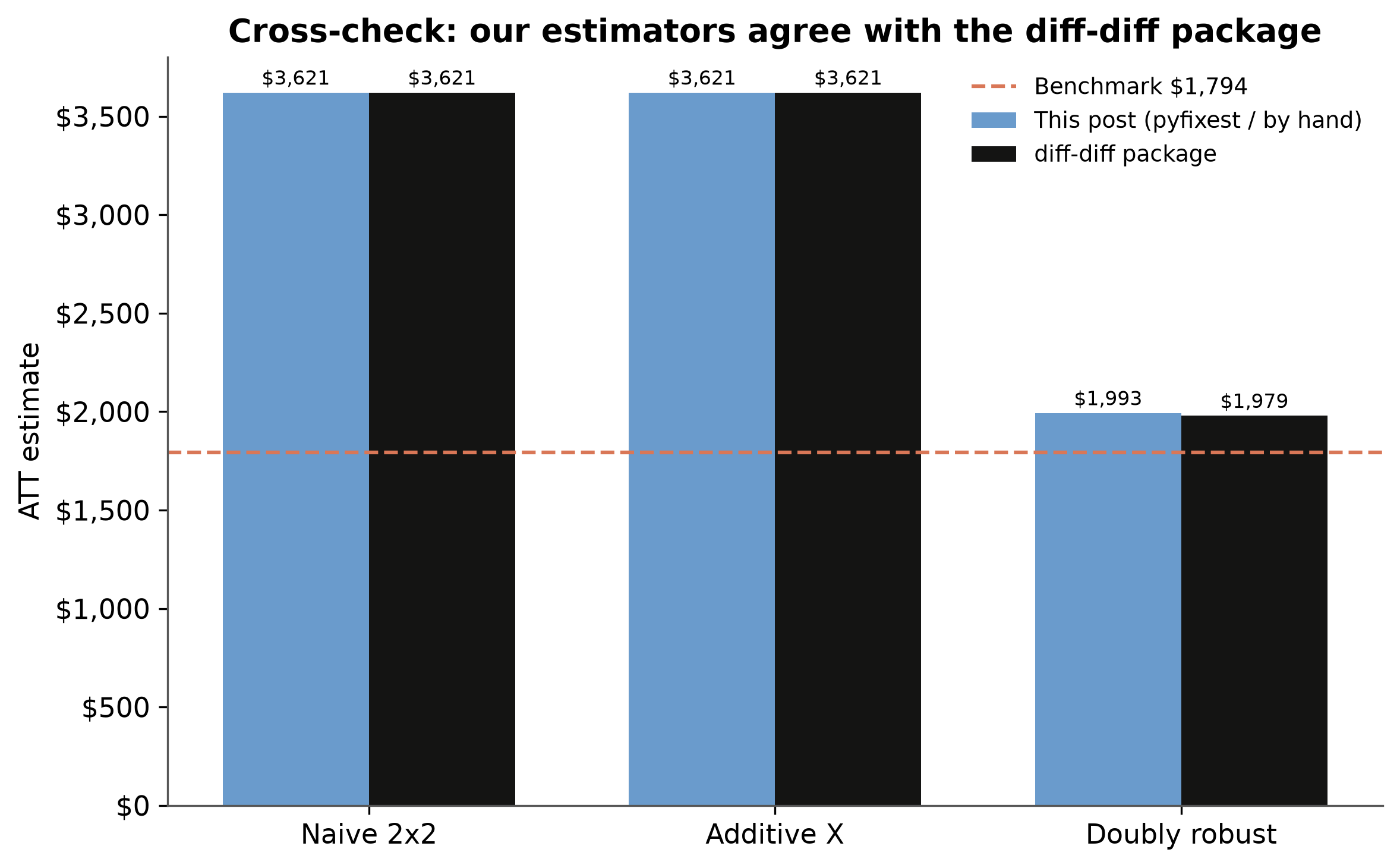
The diff-diff package matches the naive/additive numbers exactly and lands within $14 of the by-hand doubly-robust estimate.

How much should we trust $1,770 over $1,711?

Trust the pattern, not the decimal

Every corrected estimate’s 95% CI spans roughly $400 to $3,100; the benchmark itself has SE ≈ $671.

The $59 gap between Spec B and Spec C is noise. What is trustworthy is the clean split: trend-ignoring specs are all wrong the same way; trend-modeling specs all move to the truth. Reliability comes from stability across specifications and across datasets, not one lucky hit.

Takeaways

1. Placement, not inclusion. Covariates in the level ($3,621) or the effect ($3,621) are inert; in the trend ($1,711 / $1,770) they correct.
2. The common spec fails. Two-way fixed effects with additive controls is exactly the one that cannot move.
3. Two philosophies agree. Outcome regression and propensity reweighting both land near the $1,794 truth.
4. Report uncertainty honestly. Wide CIs mean the pattern is the finding, not a ranking of corrected estimates.

Resources

• Full tutorial: carlos-mendez.org/post/python_did_covariates_lalonde
• Intro to DiD: carlos-mendez.org/post/python_did
• Source: Cunningham, Covariates, diff in diff and LaLonde test, Scott’s Mixtape Substack
• RCT-vs-observational benchmarks: rctvsobs.org

Packages: pyfixest, diff-diff, causaldata.

Thank you

carlos-mendez.org