Bouncing Back Better?

Evaluating the economic impact of the 2004 Aceh tsunami

−7.9%output shock in 2005

+6.3pp/yrrecovery premium 2006–08

+18.3%synthetic-control gap by 2012

Carlos Mendez

Nagoya University (GSID)

June 12, 2026

The Tension

Act I

A magnitude-9.1 quake, a wave 9 km inland, and ~130,000 lives lost in one province

A third of Aceh’s coastline, flooded in one morning. Then the largest disaster-reconstruction effort ever — about USD 7.0 billion, well spent.

A decade later: was Aceh richer or poorer than without the wave?

The hook is the genuine ambiguity. Catastrophe destroys; well-spent aid rebuilds — which force won? The aid came through an unusually low-corruption agency, worth roughly 150% of Aceh’s damages, spent unusually well. The point of the talk is not just “what happened” but “how could you ever measure it credibly”.

You only ever observe the world where the tsunami did happen

To answer it, we need Aceh’s counterfactual — the output it would have had with no tsunami. That world is never observed; it must be estimated.

Our target is the ATT — the average effect of the treatment on the treated:

\[\text{ATT} = E[\,Y(1) - Y(0) \mid D = 1\,]\]

The effect on the flooded districts — not on some randomly chosen district.

This is the fundamental problem of causal inference. Y(1) is observed for flooded Aceh; Y(0) is not. DiD estimates Y(0) from the control group’s trend; synthetic control estimates it from a weighted blend of donor districts. Both target the ATT.

The wave’s path was geography, not choice — that is what makes it a natural experiment

Elevation, vegetation, and offshore depth decided which coast flooded — read off satellite maps, not chosen by economics. So flooded vs spared is plausibly unrelated to a district’s economic prospects.

A note on the data. Everything here runs on synthetic, calibrated data — tuned to reproduce Heger & Neumayer (2019)’s signs, significance, and approximate magnitudes. Learn the methods, not new facts about Aceh.

Treatment is defined off DLR/ZKI and Dartmouth Flood Observatory maps made 1–5 days after the wave — exogenous geographic happenstance. The synthetic-data caveat is stated up front for honesty; Section 11 of the post audits it column by column.

Six paths a shocked economy can take

After the wave, Aceh could have landed anywhere on a menu of trajectories — measured against the output it would have had with no tsunami (the dotted counterfactual).

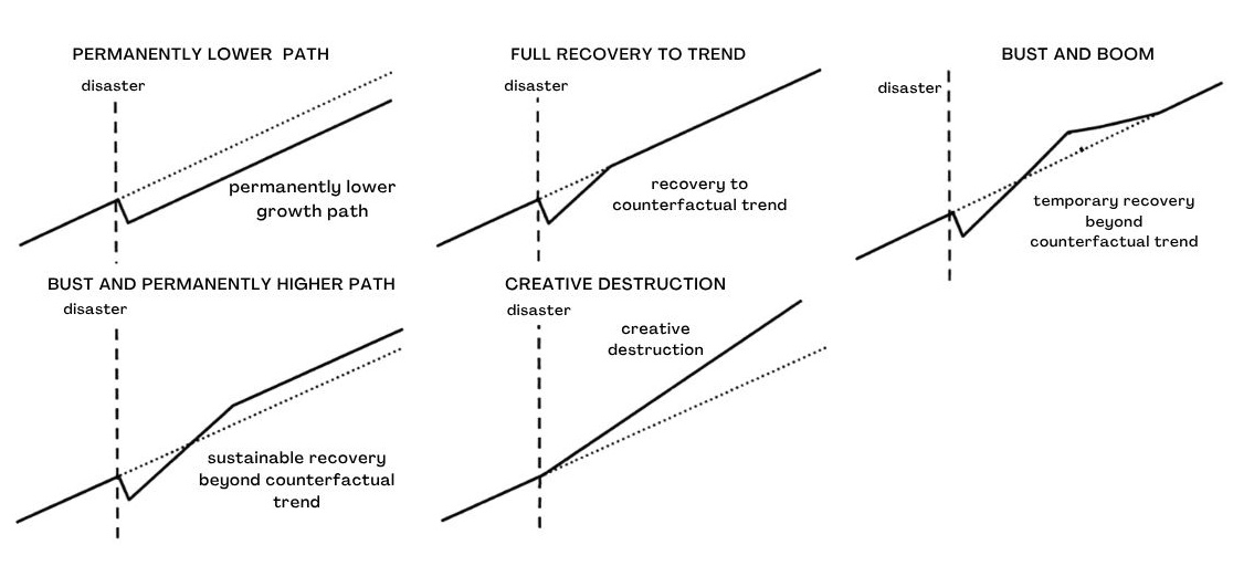
A typology of post-disaster recovery paths, each plotted against its no-disaster counterfactual trend: permanently lower path, full recovery to trend, bust and boom, bust and permanently higher path, and creative destruction.

Which one did Aceh take? Act II finds out.

The conceptual menu. A disaster can leave a region permanently poorer, exactly back on trend, temporarily above then back (bust and boom), permanently above (“build back better” — sustainable recovery beyond the counterfactual), or trigger a wave of upgrading (creative destruction). The whole investigation is about which archetype fits Aceh — the answer, foreshadowed here, is the permanently-higher path.

The Investigation

Act II

One disaster, measured at two grains — district GDP and sub-district night-lights

District GDP

• 125 Sumatran districts
• annual, 1999–2012 (1,750 rows)
• 10 flooded Aceh districts treated
• outcome: real GDP growth (oil & gas excluded)

Sub-district night-lights

• 276 Aceh sub-districts
• satellite luminosity (DMSP-OLS, 0–63)
• continuous dose: share flooded
• outcome: log-luminosity growth

Only 10 treated units — the recurring source of statistical caution.

National GDP would barely flinch at a one-province shock, so we need sub-national data at two grains. District GDP gives the headline DiD; the finer night-lights panel lets us ask whether the harder-hit places rebounded more.

Parallel before 2005, then a dive and an overshoot

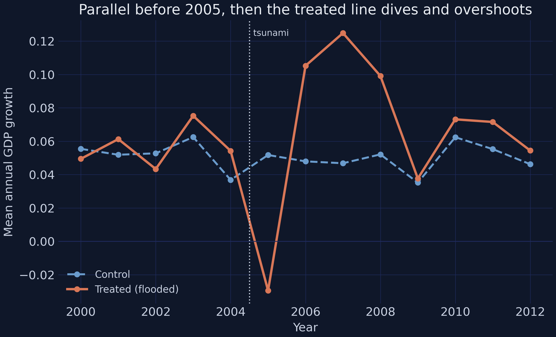
Treated (orange) vs control (blue) group-mean growth: lockstep before the tsunami, then the treated line plunges to ≈ −0.027 and overshoots to ≈ +0.124 in 2007.

This is the picture DiD was invented for. Pre-2005 the two lines move together — the visual signature of parallel trends. At the tsunami the treated line dives; then it over-shoots before settling back toward the control. The eye is convinced; the rest of the talk quantifies it and attaches a margin of error.

A single “after” hides the story

The simplest DiD splits time into before/after and takes the difference of the two changes:

\[\widehat{\text{DiD}} = \big(\bar{g}_{\text{treat, after}} - \bar{g}_{\text{treat, before}}\big) - \big(\bar{g}_{\text{ctrl, after}} - \bar{g}_{\text{ctrl, before}}\big)\]

Pooled DiD: +0.0125, insignificant (p = 0.38).

One “after” blends the 2005 crash with the 2006–08 boom — they cancel.

The pooled estimate is not wrong, it is uninformative. The fix is to let the effect vary over time — split the post period into event-time windows. That is the paper’s headline specification.

−7.9% in 2005, then +6.3 pp/yr faster in 2006–08

m = pf.feols("gdp_growth ~ D_pre + D_2005 + D_recov + D_post | district_id + year",
             data=df, vcov={"CRV1": "district_id"})
m.coef().round(4)   # D_2005 = −0.0792 · D_recov = +0.0628

Event-time window	Estimate	Conley-HAC SE	Sig.
Pre-tsunami (2003–04)	+0.0172	0.0159	ns
Tsunami (2005)	−0.0792	0.0240	***
Recovery (2006–08)	+0.0628	0.0244	**
Post-recovery (2009–12)	+0.0114	0.0146	ns

Flat pre-trend → parallel trends holds. The gain persists but doesn’t compound → a permanently higher path.

Three takeaways. The pre-tsunami coefficient is small and insignificant — parallel trends survives its formal placebo. The 2005 coefficient is −0.0792 (≈ 8% slower the year the wave hit). The recovery coefficient is +0.0628; three years of that premium more than erase the one-year loss. This is the paper’s signature “recovery beyond the counterfactual trend”.

The event study shows why the pooled average misled

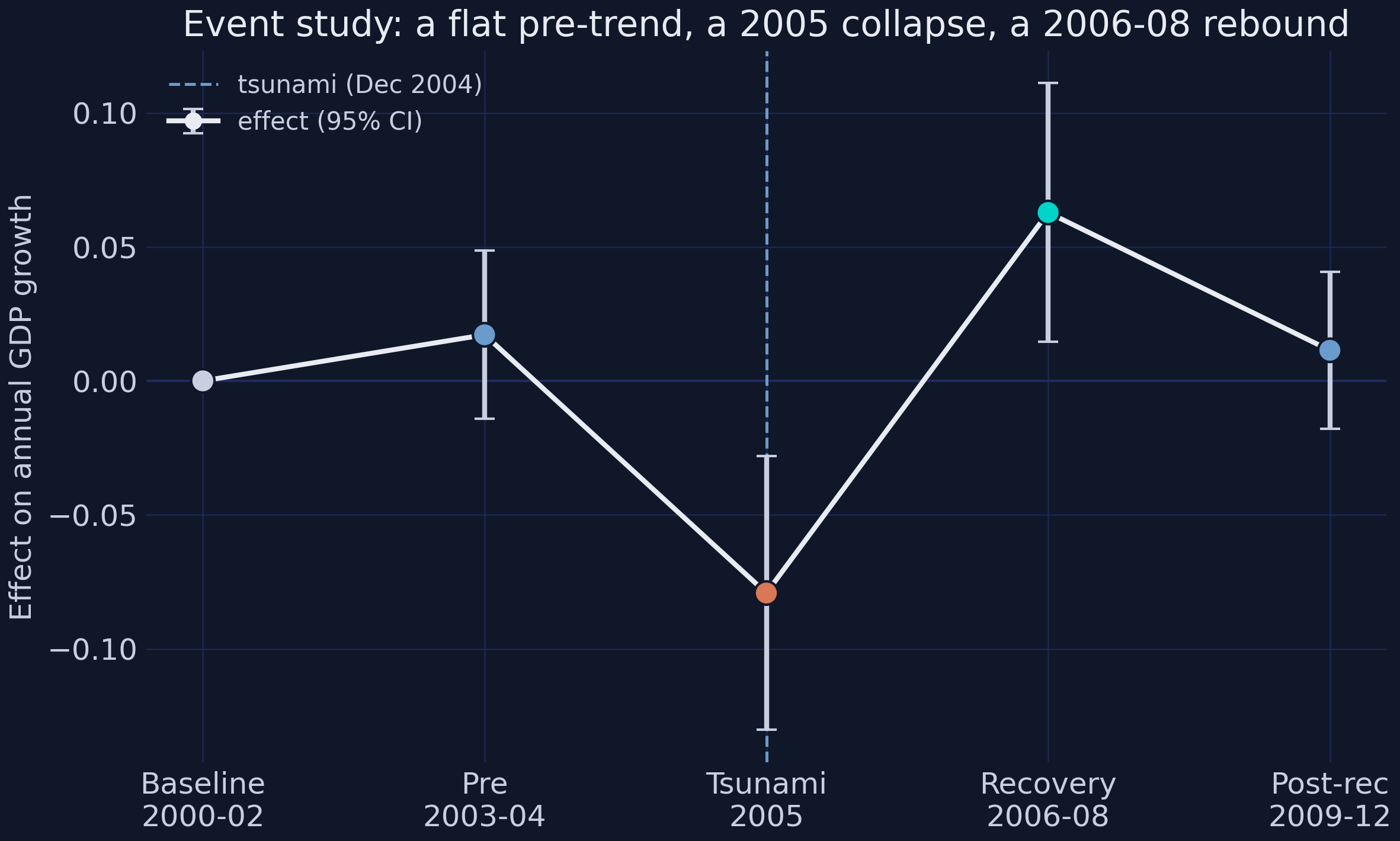
Treated-minus-control effect by period (95% CIs): baseline and pre-trend sit on zero, 2005 collapses to −0.079, recovery rebounds to +0.063, then drifts back but stays positive.

The single “after” dummy averaged the deep-negative 2005 point with the high recovery point and got a muted, insignificant number. The event study shows the whole arc — a flat pre-trend (identification visibly satisfied), a sharp collapse, a significant rebound, and a persistent higher level.

Not a denominator artifact — per-capita recovery is even larger

A worry: maybe “growth” rose only because population fell (130,000 deaths and displacement). Re-running the DiD on GDP per capita:

+0.0827

recovery coefficient on per-capita growth, p < 0.01 — output per person rose, not just totals

In per-capita terms there is no significant 2005 loss (output and population fell together that year), but the recovery gain strengthens to +0.0827. Fewer people then shared a rebuilt, better-capitalized economy. The effect survives dividing by population.

The harder-hit rebounded more — and only the worst-hit fifth significantly

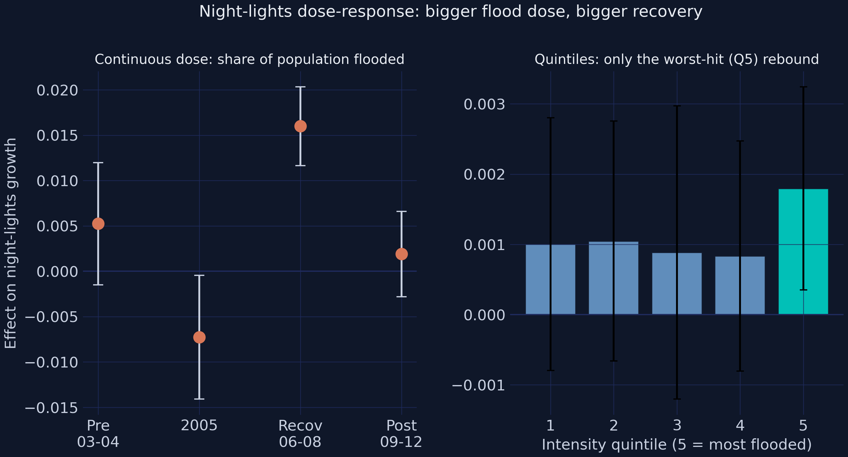
Night-lights dose-response: continuous period effects (left) and effect by flood-intensity quintile (right) — only Q5, the most heavily flooded sub-districts, rebounds significantly.

Quintile	Q1	Q2	Q3	Q4	Q5 (worst-hit)
Recovery effect	+0.0010	+0.0010	+0.0009	+0.0008	+0.0018**

Each unit of population-share flooded buys +0.016/year extra luminosity growth in recovery (p < 0.001). But the average is not spread evenly — only the top intensity quintile shows a significant rebound. The effect concentrates exactly where the damage, and therefore the reconstruction spending, was greatest.

A synthetic Aceh, built from 76 donors, tracks the pre-2005 path almost exactly

Synthetic control picks non-negative weights \(w\) that sum to one to minimize pre-treatment mismatch:

\[w^{\ast} = \arg\min_{w}\ (X_1 - X_0 w)^{\top} V (X_1 - X_0 w) \quad \text{s.t.}\quad w_j \ge 0,\ \textstyle\sum_j w_j = 1\]

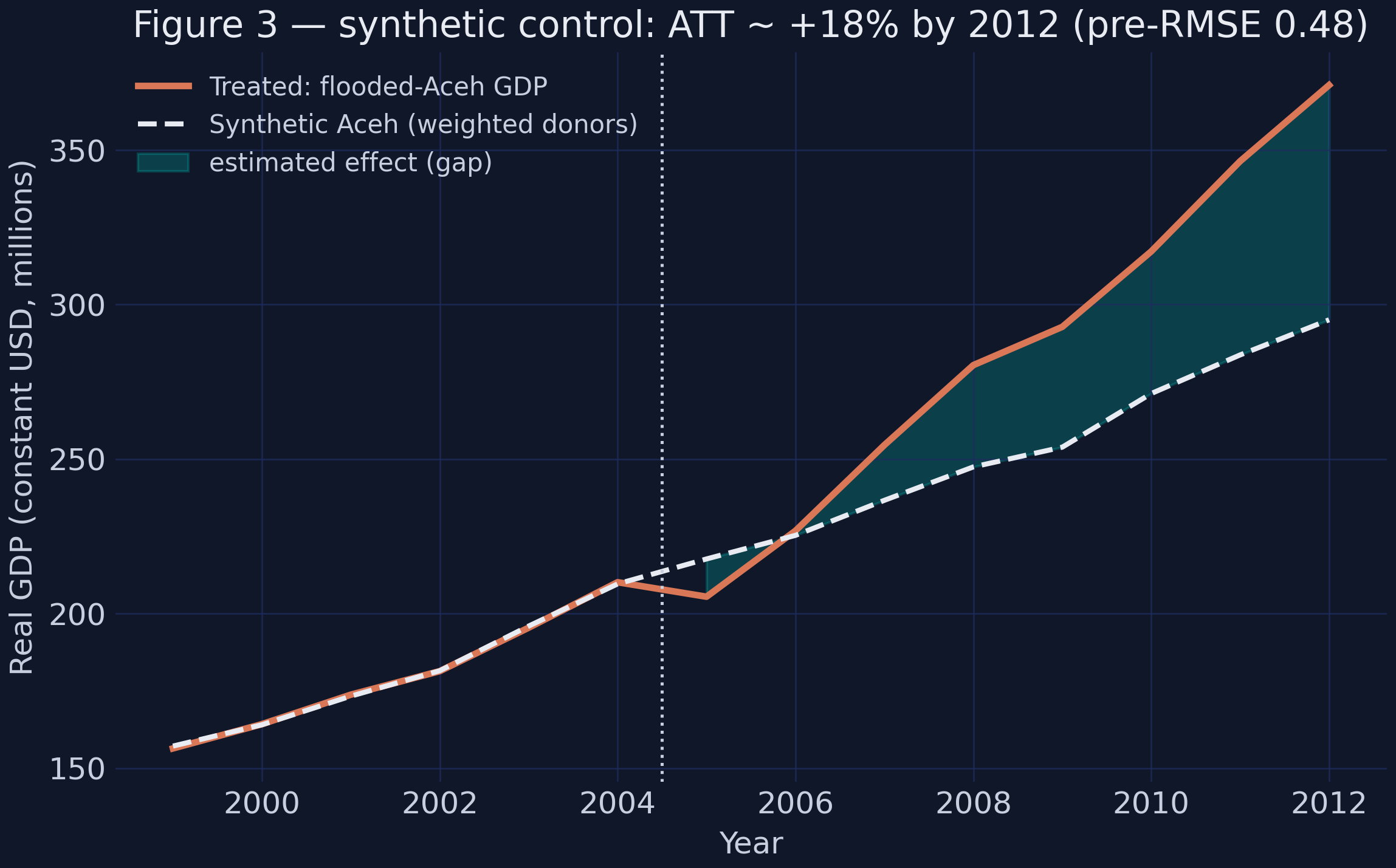
Synthetic Aceh tracks the real path before 2005 (pre-RMSE 0.485); afterward the actual line pulls above.

A pre-RMSE of 0.485 against GDP levels near 200 means synthetic Aceh shadows the real thing almost perfectly before 2005 — which is what licenses trusting it as a counterfactual afterward. The top weight is only 0.13; the counterfactual rests on many modest donors, not one look-alike.

+18.3% above its no-tsunami twin by 2012 — and the gap opens only after the wave

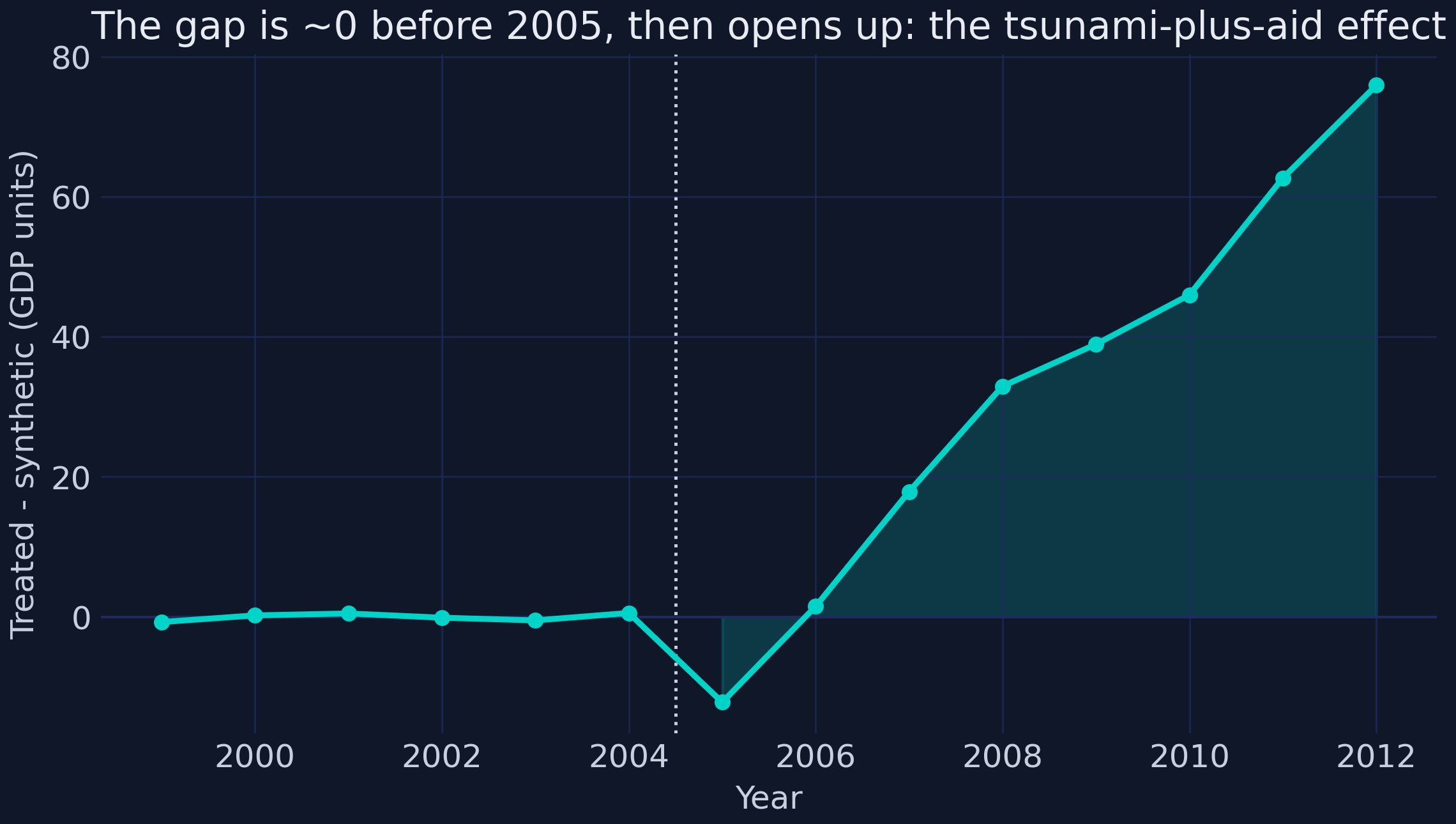
The treated-minus-synthetic gap: indistinguishable from zero before 2005, then steadily positive.

Two very different methods — DiD and synthetic control — now agree: flooded Aceh ended materially above where it was heading.

By 2012 actual Aceh is at 370.9 vs the synthetic 295.0 — a +18.3% gap. The gap plot isolates the divergence: zero before treatment, opening afterward. Triangulation across independent methods is a far stronger claim than any one method alone.

All 10 treated units sit in one corner of the map

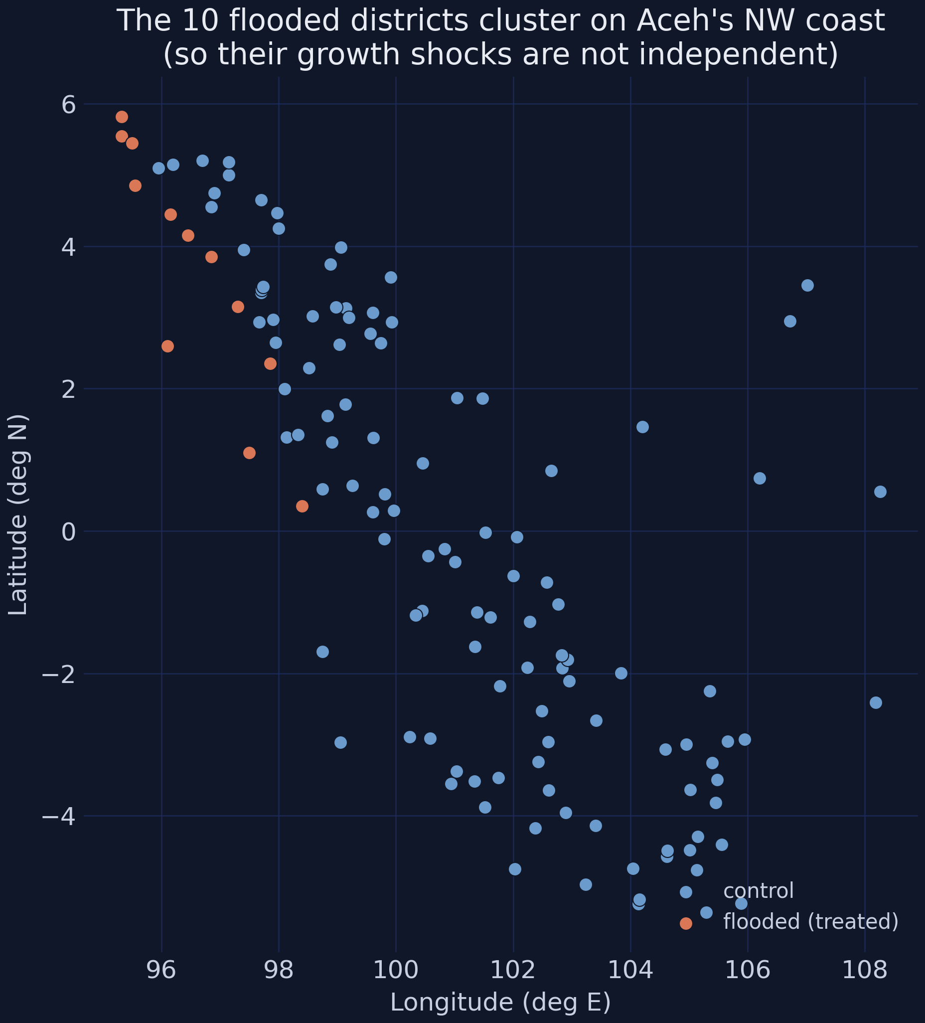
Longitude–latitude scatter of every Sumatran district: the 10 flooded (treated) units, in orange, cluster on Aceh’s far north-west coast.

Near things are more related than distant things — their growth shocks are not independent draws.

When treated units are packed together, a good monsoon, a regional price swing, or the reconstruction boom itself hits them together. The default standard error assumes independence, so it counts more truly-independent information than the data contain — and reports SEs that are too small.

The point estimate never moved — only our honesty about it did

Moran’s I on the residuals is +0.065 (permutation p = 0.003): nearby districts’ growth is significantly correlated. The fix is a Conley spatial-HAC standard error.

Recovery effect	Estimate	Naive SE	Conley-HAC SE	t(HAC)
2006–08	+0.0628	0.0146	0.0244	+2.57

Same +0.0628 in every column. The SE inflates 1.68× — downgrading a spurious *** to an honest **.

Under the naive error the recovery effect would have a t above 4 and look significant at 1%. Under the honest Conley-HAC error its t is 2.57 — significant at 5%, not 1%. A careless analyst would have overstated the confidence threefold. The SE is stable across the 25–100 km cutoff range the paper uses.

The Resolution

Act III

Four methods, one story: recovery beyond the counterfactual trend

• DiD — −7.9% in 2005, +6.3 pp/yr in 2006–08, on a permanently higher path
• Event study — flat pre-trend, sharp collapse, significant rebound
• Night-lights — the dose-response: only the worst-hit quintile rebounds
• Synthetic control — +18.3% above the no-tsunami Aceh by 2012

Triangulation, not a single regression, is what makes the claim credible.

Four tools built on different assumptions all point the same way. That convergence — not the precision of any one estimate — is the strongest part of the evidence.

Well-governed mega-reconstruction can bend a poor region’s path upward

The lesson is not “disasters are good” — 130,000 people died. It is that a localized catastrophe followed by large, well-spent aid can leave a poor region permanently better off.

Aid ≈ 150% of damages · low-corruption agency · “built back better.”

That combination — not the wave — bent the path upward.

For disaster policy the design lesson matters as much as the result: a credible evaluation needs exogenous exposure (geography, not choice), a finer-than-national unit of analysis, and spatially honest standard errors.

The strongest objection — and the answer

Objection. The data are synthetic, and there are only 10 treated districts — point estimates are fragile, standard errors wide.

Response.

• Synthetic data are calibrated to the paper — audited column by column.
• Small-N met head-on: flat pre-trend, null placebo, Conley-HAC errors.
• Caveats narrow the claim — they don’t overturn it.

Steelman first: this is a single, exceptionally well-funded case study on simulated data with a tiny treatment group. The honest reply is that every credibility check — placebo, pre-trend, spatial inference — has been run and survived, and the conclusion is stated as evidence about well-governed mega-reconstruction, not disaster aid in general.

Five numbers to remember

Number	Value
2005 output shock	−0.0792***
2006–08 recovery premium (per year)	+0.0628**
Synthetic-control gap by 2012	+18.3%
Moran’s I (spatial autocorrelation)	+0.065
Recovery SE: naive → Conley-HAC	0.0146 → 0.0244

And five lessons: let evolving effects evolve · triangulate · satellite data unlock localized questions · clustered treatment needs honest inference · mind the small print.

Close on the numbers, then the five lessons. One: the pooled 2×2 was an insignificant +0.0125 — only event-time windows revealed the −0.079 collapse and +0.063 overshoot, so let evolving effects evolve. Two: DiD, event study, dose-response, and synthetic control all pointed the same way; agreement beats any one estimate. Three: night-lights exposed a dose-response invisible at the district grain. Four: Conley spatial errors downgraded the recovery from a spurious *** to an honest ** without touching the point estimate. Five: ten treated districts on synthetic data, identified by an assumption — strong evidence, stated with its caveats. Next steps in the post: staggered-adoption DiD estimators, prediction intervals for the synthetic control, a wider donor pool.

A poor region, well-governed reconstruction, a permanently higher path.