A Beginner's Guide to Causal Inference with DoWhy in Python
Abstract
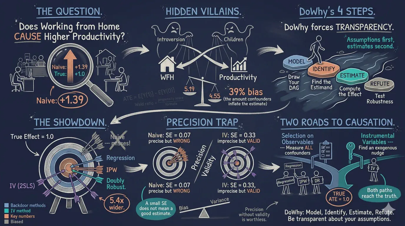
Observational data routinely conflate causation with selection: more productive people may simply choose to work from home, making naive comparisons misleading whenever confounders are present. This tutorial introduces causal inference through DoWhy, a Python library, with the objective of recovering a known treatment effect from observational data and showing how its four-step framework — Model, Identify, Estimate, Refute — keeps causal assumptions separate from statistical estimation. The analysis uses a simulated observational dataset of 5,000 employees in which the true average treatment effect (ATE) of working from home on productivity is fixed at 1.0 points; treatment is non-randomly assigned through two confounders (introversion and number of children), and a subway-disruption instrument satisfies the exclusion restriction by construction. Four estimators are applied — linear regression, inverse probability weighting (IPW), doubly robust estimation (AIPW), and instrumental variables (2SLS) — and compared against the naive difference in means. The naive estimate of 1.39 overshoots the truth by 39%, while the backdoor methods recover the ATE closely (regression 1.0051, SE 0.0614; IPW 1.0275, SE 0.0754; AIPW 1.0115, SE 0.0623) and IV returns 0.8881 with a much larger SE of 0.3303 despite a strong first-stage F of 293.0; refutation tests (placebo ≈ 0, random common cause and data subset ≈ 1.0) confirm stability. The results show that explicit identification and method comparison — not precision alone — separate genuinely causal estimates from confidently wrong ones.
Overview
Does working from home actually make employees more productive, or do more productive people simply choose to work from home? This is the fundamental challenge of causal inference: distinguishing genuine cause-and-effect relationships from misleading correlations driven by confounding variables.
In this tutorial, we use simulated observational data where the true causal effect is known (ATE = 1.0) to demonstrate how DoWhy — a Python library for causal inference — helps us recover the correct answer. We walk through DoWhy’s four-step framework (Model, Identify, Estimate, Refute) and apply four estimation methods: Linear Regression, Inverse Probability Weighting (IPW), Doubly Robust estimation (AIPW), and Instrumental Variables (2SLS).
This tutorial is inspired by the DataCamp introduction to Causal AI using DoWhy and builds on a more comprehensive DoWhy tutorial with the Lalonde dataset that covers five estimation methods with real-world data.
Learning objectives:
- Understand why naive comparisons can be misleading when confounders are present
- Learn DoWhy’s four-step causal inference framework (Model, Identify, Estimate, Refute)
- Define a causal graph (DAG) that encodes your assumptions about what causes what
- Distinguish two identification strategies: selection on observables (backdoor criterion) and instrumental variables
- Estimate causal effects using four methods and compare them against the known truth
- Assess robustness of estimates using automated refutation tests
Key concepts at a glance
The post leans on a small vocabulary repeatedly. The rest of the tutorial assumes you can move between these terms quickly. Each concept below has three parts. The definition is always visible. The example and analogy sit behind clickable cards: open them when you need them, leave them collapsed for a quick scan. If a later section mentions “backdoor criterion” or “exclusion restriction” and the term feels slippery, this is the section to re-read.
1. Confounder. A variable that affects both the treatment and the outcome. Confounders create a backdoor path that biases naive comparisons. Without adjustment, we cannot distinguish the treatment’s effect from the confounder’s effect.
Example
In our simulated data, introversion and num_children are the two confounders. Introverts both prefer working from home AND tend to be more productive. The naive WFH-vs-office gap is 1.39 productivity points, but the true effect is only 1.0. The 0.39 gap is confounder bias.
Analogy
A pair of children who both eat ice cream and both get sunburned. The ice-cream truck did not cause the sunburn. A third lurking variable — sunny weather — caused both. The confounder is that sun.
2. Causal graph (DAG). A directed acyclic graph that encodes assumptions about which variables cause which others. Nodes are variables. Arrows point from cause to effect. The DAG is DoWhy’s “Step 1” (Model). It is the assumption layer the rest of the analysis stands on.
Example
In this tutorial the DAG has arrows from introversion and num_children into both work_from_home and productivity, plus a direct arrow from work_from_home to productivity. That single direct arrow is the causal effect we want.
Analogy
A wiring diagram for a kitchen appliance. The diagram does not tell you whether the appliance works. It tells you which wires connect to which terminals. If you trust the diagram, you can predict what happens when a wire breaks.
3. Backdoor criterion. An identification rule. If a set of variables blocks every backdoor path from treatment to outcome, conditioning on that set identifies the causal effect. The set must not include descendants of the treatment.
Example
In our DAG, conditioning on {introversion, num_children} blocks every backdoor path from work_from_home to productivity. That is why linear regression with those controls recovers 1.0051 — close to the truth.
Analogy
Two acquaintances exchange gossip through three mutual friends. To stop the gossip from reaching one acquaintance, you do not need to interview each of them. You just need to silence one person on every route. That person is the blocking set.
4. Propensity score $e(\mathbf{x}) = P(T=1 \mid \mathbf{X}=\mathbf{x})$. The conditional probability of receiving the treatment, given the covariates. The propensity score summarizes everything in $\mathbf{X}$ that affects treatment assignment. It is the engine behind IPW and AIPW. We never observe it directly. We estimate it from the data.
Example
In our data the average propensity is about 0.66 (66.2% of employees work from home). For a high-introversion employee with two children, the propensity is much higher. For an extrovert with no children, it is much lower. IPW and AIPW both rely on this estimated function.
Analogy
A casino’s odds that the next card is dealt face-up. We do not see the casino’s algorithm. We just observe many deals and estimate the odds. Once we have them, we can reweight outcomes to undo the dealer’s bias.
5. IPW — Inverse Probability Weighting. A reweighting estimator. Each observation gets weight $1/\hat{e}(\mathbf{x})$ if treated and $1/(1-\hat{e}(\mathbf{x}))$ if control. The weighted average difference estimates the ATE. IPW is consistent if the propensity model is correct. It is sensitive to extreme propensity scores (near 0 or 1).
Example
IPW gives 1.0275 (SE = 0.0754) on our data. The bias is +0.0275 — half of one percent of an employee whose true effect is 1.0 productivity point. Compare with the naive 1.39: the bulk of the bias is gone.
Analogy
A national poll over-samples college students. To estimate the population mean, we re-weight each student by the reciprocal of how over-represented their group is. IPW does the same thing for treatment groups.
6. Doubly robust / AIPW — Augmented IPW. Combines an outcome regression with the IPW reweight, plus a correction term. Doubly robust means the estimator stays consistent if either the outcome model is correct or the propensity model is correct. Both being right is gravy. Both being wrong is the only failure mode.
Example
AIPW gives 1.0115 (SE = 0.0623) on our data. Of the four estimators (linear, IPW, AIPW, IV) it has the smallest absolute bias. The double robustness explains why: even when the outcome model leaves a little structure on the table, the IPW reweight cleans it up.
Analogy
Belt and suspenders. If the belt fails, the suspenders hold. If the suspenders fail, the belt holds. Both fail simultaneously? Time to buy new pants. AIPW is two failures away from a wardrobe malfunction.
7. Instrumental variable + exclusion restriction. An instrumental variable $Z$ is a source of variation in the treatment that affects the outcome only through the treatment. The exclusion restriction is the assumption that $Z$ has no direct effect on $Y$ except via $T$. IV identifies a Local Average Treatment Effect (LATE), not the ATE, when effects are heterogeneous.
Example
subway_disruption is the instrument here. Subway disruptions push some employees to work from home that day. The exclusion assumption says disruptions affect productivity only by changing WFH status — not directly. The 2SLS estimate is 0.8881 (SE = 0.3303). The first-stage F is 293.0, so the instrument is strong.
Analogy
A coin flip you did not ask for. Some employees got “heads” (subway broke, they had to WFH) and some got “tails”. The flip is random with respect to introversion and family size. Comparing across the flip’s outcome isolates the WFH effect — but only for the kind of employee whose WFH choice actually changes when a subway breaks.
8. Refutation tests. DoWhy’s “Step 4” (Refute). Stress tests that probe the estimate’s stability. Common refuters include placebo treatment (replace the real treatment with a random one and re-estimate; expect zero), random common cause (add a fake confounder; expect the estimate not to move), and data subset (re-estimate on a random subsample; expect the estimate to stay close).
Example
After estimating 1.0115 with AIPW we run all three refuters. The placebo refuter returns ~0 (good). The random-common-cause refuter returns ~1.0 (good). The data-subset refuter returns ~1.0 across multiple random subsamples (good). The estimate survives.
Analogy
Stress-testing a recipe. Add a teaspoon of an irrelevant ingredient — does the dish still taste right? Use half the flour — does it still rise? A recipe that survives those small perturbations is more trustworthy than one that does not.
The problem: confounding bias
Imagine a company wants to know if its work-from-home (WFH) policy improves productivity. They collect data on 5,000 employees and compare productivity between those who work from home and those who go to the office.
The naive comparison shows that WFH employees are 1.39 productivity points higher. But the true causal effect is only 1.0 points. What went wrong?
The answer is confounding. Two variables — introversion and number of children — affect both the decision to work from home and productivity itself:
- Introverts prefer working from home (fewer social interruptions) AND are independently more productive (they focus better in quiet environments)
- Parents with more children prefer WFH for flexibility AND tend to have slightly lower productivity (more distractions at home)
Because introverts self-select into WFH and are also more productive, the naive comparison overestimates the true effect by 39%.
DoWhy’s four-step framework
Most statistical software lets you jump from data to estimates without stating your assumptions. DoWhy takes a different approach: it organizes every causal analysis into four explicit steps.
graph LR
    A["1. Model<br/>Define causal graph"] --> B["2. Identify<br/>Find estimand"]
    B --> C["3. Estimate<br/>Compute effect"]
    C --> D["4. Refute<br/>Test robustness"]
    style A fill:#6a9bcc,stroke:#141413,color:#fff
    style B fill:#d97757,stroke:#141413,color:#fff
    style C fill:#00d4c8,stroke:#141413,color:#fff
    style D fill:#8b5cf6,stroke:#141413,color:#fff
| Step | Question | What you do |
|---|---|---|
| Model | What are my causal assumptions? | Draw a DAG (Directed Acyclic Graph) showing which variables cause which |
| Identify | Can I compute the causal effect from data? | DoWhy checks if your graph allows identification via backdoor, IV, or front-door criteria |
| Estimate | What is the numerical value of the causal effect? | Apply statistical methods (regression, IPW, doubly robust, IV) |
| Refute | Is this estimate robust? | Run automated tests: placebo treatment, random confounder, data subsets |
The key insight is that identification (step 2) is a causal problem that depends on your assumptions, while estimation (step 3) is a statistical problem that depends on your data. DoWhy keeps them separate.
Setup and imports
import warnings
warnings.filterwarnings("ignore")

import numpy as np
import pandas as pd
import matplotlib.pyplot as plt
from sklearn.linear_model import LogisticRegression, LinearRegression
from dowhy import CausalModel
# Configuration
RANDOM_SEED = 42
np.random.seed(RANDOM_SEED)

N = 5000           # sample size
TRUE_ATE = 1.0     # known true effect

TREATMENT = "work_from_home"
OUTCOME = "productivity"
CONFOUNDERS = ["introversion", "num_children"]
INSTRUMENT = "subway_disruption"
The data: simulated observational study
We simulate data where the true causal effect is known (ATE = 1.0), so we can verify whether each method recovers the correct answer. This is the gold standard for learning causal inference: if a method cannot recover the truth when we know it, we should not trust it on real data where we do not.
Data generating process
The data generating process (DGP) defines how each variable is generated. Think of it as the “rules of the universe” in our simulation:
def generate_wfh_data(n, seed):
    rng = np.random.default_rng(seed)

    # Confounders (affect BOTH treatment and outcome)
    introversion = rng.normal(5, 1.5, n)
    num_children = rng.poisson(1.5, n)

    # Instrument (affects treatment ONLY)
    subway_disruption = rng.binomial(1, 0.4, n)

    # Treatment: who works from home? (observational, not random!)
    logit_p = -1.5 + 0.3*introversion + 0.2*num_children + 1.0*subway_disruption
    prob_wfh = 1 / (1 + np.exp(-logit_p))
    work_from_home = rng.binomial(1, prob_wfh)

    # Outcome: productivity (note: subway_disruption does NOT appear here)
    noise = rng.normal(0, 2, n)
    productivity = (50
                    + 1.0 * work_from_home      # TRUE causal effect
                    + 0.8 * introversion         # confounder effect
                    - 0.5 * num_children         # confounder effect
                    + noise)

    return pd.DataFrame({
        "work_from_home": work_from_home,
        "productivity": productivity,
        "introversion": introversion,
        "num_children": num_children,
        "subway_disruption": subway_disruption,
    })

df = generate_wfh_data(N, RANDOM_SEED)
Notice three critical features of this DGP:
- Treatment is NOT random. More introverted employees and those with more children are more likely to choose WFH. This is what makes it observational data.
- Confounders affect both treatment and outcome. Introversion increases both the probability of WFH (logit coefficient = 0.3) and productivity directly (coefficient = 0.8).
- The instrument satisfies the exclusion restriction.
subway_disruptionappears in the treatment equation (coefficient = 1.0) but NOT in the outcome equation. It only affects productivity through WFH choice.
Dataset shape: (5000, 5)
Treatment prevalence: 66.2% work from home

       work_from_home  productivity  introversion  num_children  subway_disruption
count         5000.00       5000.00       5000.00       5000.00         5000.00
mean             0.66         53.88          4.97          1.50            0.42
std              0.47          2.49          1.50          1.22            0.49
min              0.00         43.90         -0.47          0.00            0.00
max              1.00         62.52         10.18          8.00            1.00
About two-thirds of employees in our sample work from home, and 42% live near the disrupted subway line. Productivity scores range from about 44 to 63 with a mean of 53.88.
Exploratory data analysis
The naive estimate
The simplest approach is to compare average productivity between the two groups:
mean_wfh = df[df[TREATMENT] == 1][OUTCOME].mean()
mean_office = df[df[TREATMENT] == 0][OUTCOME].mean()
naive_ate = mean_wfh - mean_office
Mean productivity (WFH):    54.35
Mean productivity (Office): 52.97
Naive ATE (difference):     1.39
True ATE:                   1.00
Bias (naive - true):        0.39
The naive estimate of 1.39 overshoots the true effect of 1.0 by 39%. This upward bias occurs because the WFH group contains more introverts, who are independently more productive. The naive comparison attributes all of the productivity difference to working from home, when in fact part of it is due to personality differences.
Visualizing the confounding
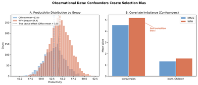
Panel A shows the productivity distributions for office (blue) and WFH (orange) workers. The WFH distribution is shifted to the right, but not all of this shift is causal — part of it reflects the higher introversion of WFH workers. The dotted line shows where the office distribution would shift if only the true causal effect (1.0) were acting.
Panel B reveals the covariate imbalance: WFH employees have higher introversion (5.19 vs 4.55) and more children (1.58 vs 1.33) than office workers. This imbalance is the fingerprint of self-selection and the source of confounding bias.
Step 1: Model — Define the causal graph
The first step in DoWhy is to encode your causal assumptions as a Directed Acyclic Graph (DAG). A DAG is simply a diagram showing which variables cause which, with arrows pointing from causes to effects.
What is a DAG?
A DAG has three properties:
- Directed: Each arrow points in one direction (cause → effect)
- Acyclic: You cannot follow arrows in a circle back to where you started
- Graph: Variables are nodes, causal relationships are edges (arrows)
Our causal graph
graph LR
    I["Introversion<br/>(Confounder)"] --> T["Work from Home<br/>(Treatment)"]
    I --> Y["Productivity<br/>(Outcome)"]
    C["Num. Children<br/>(Confounder)"] --> T
    C --> Y
    Z["Subway Disruption<br/>(Instrument)"] --> T
    T --> Y
    style I fill:#999,stroke:#141413,color:#fff
    style C fill:#999,stroke:#141413,color:#fff
    style Z fill:#00d4c8,stroke:#141413,color:#fff
    style T fill:#d97757,stroke:#141413,color:#fff
    style Y fill:#6a9bcc,stroke:#141413,color:#fff
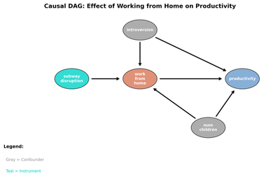
Three types of variables appear in our DAG:
- Confounders (gray): Introversion and num_children have arrows pointing to both treatment and outcome. They create “backdoor paths” that confound the naive comparison.
- Instrument (teal): Subway disruption has an arrow to treatment but not to outcome. It provides exogenous variation in WFH choice — employees near the closed subway line are forced to work from home regardless of their personality or family situation.
- Treatment and Outcome (orange and blue): The arrow from treatment to outcome represents the causal effect we want to estimate.
Creating the CausalModel
model = CausalModel(
    data=df,
    treatment=TREATMENT,
    outcome=OUTCOME,
    common_causes=CONFOUNDERS,
    instruments=[INSTRUMENT],
)
DoWhy creates an internal graph object that it uses in subsequent steps. The common_causes argument tells DoWhy which variables are confounders, and instruments identifies variables that affect treatment but not outcome.
Step 2: Identify — Find the estimand
Identification answers the question: Can we express the causal effect as something we can compute from data? This is purely a theoretical step — it depends on the graph, not the data.
identified_estimand = model.identify_effect(proceed_when_unidentifiable=True)
print(identified_estimand)
DoWhy automatically discovers two valid identification strategies:
Strategy 1: Backdoor criterion (selection on observables)
$$ ATE = E\left[\frac{\partial}{\partial T} E[Y \mid T, X_1, X_2]\right] $$
where \(T\) is work_from_home, \(Y\) is productivity, \(X_1\) is introversion, and \(X_2\) is num_children.
In plain language: if we condition on all confounders (introversion and num_children), the remaining association between treatment and outcome is the causal effect. This is called selection on observables because it assumes we have measured all variables that simultaneously affect treatment and outcome.
The critical assumption is unconfoundedness: there are no unmeasured common causes of WFH choice and productivity. If this holds, conditioning on the observed confounders blocks all backdoor paths.
Strategy 2: Instrumental variable
$$ATE = \frac{E\left[\frac{\partial Y}{\partial Z}\right]}{E\left[\frac{\partial T}{\partial Z}\right]}$$
where \(Z\) is subway_disruption.
In plain language: divide the effect of the instrument on the outcome (reduced form) by the effect of the instrument on the treatment (first stage). The instrument provides a “natural experiment” — variation in WFH choice that is not driven by confounders.
The critical assumption is the exclusion restriction: subway_disruption affects productivity only through its effect on WFH choice, not directly. In our simulation, this holds by construction.
Step 3: Estimate — Compute the causal effect
Now we apply four estimation methods. Methods 1–3 use the backdoor criterion (selection on observables), while Method 4 uses the instrumental variable strategy.
Method 1: Linear Regression (backdoor adjustment)
The simplest approach: include confounders as control variables in a regression.
$$Y_i = \beta_0 + \beta_1 T_i + \beta_2 X_{1i} + \beta_3 X_{2i} + \varepsilon_i$$
The coefficient \(\beta_1\) is the causal effect, provided the model is correctly specified and all confounders are included.
estimate_reg = model.estimate_effect(
    identified_estimand,
    method_name="backdoor.linear_regression",
    confidence_intervals=True,
)
Estimated ATE: 1.0051
Robust SE (HC1): 0.0614
95% CI: [0.8847, 1.1255]
Bias from true (1.0): 0.0051
Linear regression recovers the true effect almost exactly (bias = 0.5%). The robust standard error (HC1) of 0.0614 accounts for potential heteroskedasticity — the possibility that the variance of productivity differs between WFH and office workers. The 95% CI comfortably contains the true ATE of 1.0. In practice, we rarely know the true functional form, which is why we use multiple methods.
Method 2: Inverse Probability Weighting (IPW)
IPW takes a completely different approach. Instead of modeling the outcome, it models the treatment assignment mechanism (who gets treated and why).
The idea: weight each observation by the inverse of the probability of receiving its actual treatment, given confounders. This creates a pseudo-population where treatment is independent of confounders — mimicking what would happen in a randomized experiment.
$$\widehat{ATE}_{IPW} = \frac{1}{N}\sum_{i=1}^{N}\left[\frac{T_i Y_i}{\hat{e}(X_i)} - \frac{(1 - T_i) Y_i}{1 - \hat{e}(X_i)}\right]$$
where \(\hat{e}(X_i) = P(T_i = 1 \mid X_i)\) is the propensity score — the predicted probability of working from home given the confounders.
estimate_ipw = model.estimate_effect(
    identified_estimand,
    method_name="backdoor.propensity_score_weighting",
    method_params={"weighting_scheme": "ips_weight"},
)
Estimated ATE: 1.0275
Robust SE (influence function): 0.0754
95% CI: [0.8797, 1.1754]
Bias from true (1.0): 0.0275
IPW recovers the true effect with a bias of only 2.8%. Its robust SE (0.0754) is computed from the influence function of the Hajek (stabilized) estimator, which is inherently robust to heteroskedasticity. The SE is slightly larger than regression’s (0.0614) because IPW discards the outcome model entirely and relies solely on propensity scores — using less information means more uncertainty. It relies on correct specification of the propensity score model (the probability of treatment given confounders) rather than the outcome model.
Method 3: Doubly Robust (AIPW)
What if we are not sure whether the outcome model or the propensity score model is correctly specified? The doubly robust estimator (also called Augmented IPW or AIPW) combines both models. It is consistent if either model is correctly specified — hence “doubly robust.”
$$\widehat{ATE}_{DR} = \frac{1}{N}\sum_{i=1}^{N}\left[(\hat{\mu}_1(X_i) - \hat{\mu}_0(X_i)) + \frac{T_i(Y_i - \hat{\mu}_1(X_i))}{\hat{e}(X_i)} - \frac{(1-T_i)(Y_i - \hat{\mu}_0(X_i))}{1 - \hat{e}(X_i)}\right]$$
where \(\hat{\mu}_1(X_i)\) and \(\hat{\mu}_0(X_i)\) are the predicted outcomes under treatment and control, and \(\hat{e}(X_i)\) is the propensity score.
# Fit propensity score model
ps_model = LogisticRegression(max_iter=1000, random_state=RANDOM_SEED)
ps_model.fit(df[CONFOUNDERS], df[TREATMENT])
ps = ps_model.predict_proba(df[CONFOUNDERS])[:, 1]

# Fit outcome models for each treatment group
outcome_model_1 = LinearRegression().fit(
    df[df[TREATMENT] == 1][CONFOUNDERS], df[df[TREATMENT] == 1][OUTCOME])
outcome_model_0 = LinearRegression().fit(
    df[df[TREATMENT] == 0][CONFOUNDERS], df[df[TREATMENT] == 0][OUTCOME])

# Predicted potential outcomes
mu1 = outcome_model_1.predict(df[CONFOUNDERS])
mu0 = outcome_model_0.predict(df[CONFOUNDERS])

# AIPW formula
T = df[TREATMENT].values
Y = df[OUTCOME].values
dr_ate = np.mean(
    (mu1 - mu0)
    + T * (Y - mu1) / ps
    - (1 - T) * (Y - mu0) / (1 - ps)
)
Estimated ATE: 1.0115
Robust SE (influence function): 0.0623
95% CI: [0.8893, 1.1336]
Bias from true (1.0): 0.0115
The doubly robust estimate of 1.0115 (bias = 1.2%) sits between regression and IPW. Its robust SE (0.0623) is nearly identical to regression’s (0.0614), which makes sense: when both models are correctly specified, DR achieves the semiparametric efficiency bound — the smallest possible variance for any regular estimator of the ATE. In practice, doubly robust is often the preferred method because it provides insurance against misspecification of either model while maintaining excellent precision.
Method 4: Instrumental Variables (2SLS)
Methods 1–3 all rely on selection on observables — the assumption that we have measured all confounders. But what if there are unmeasured confounders? For example, what if “self-discipline” affects both WFH choice and productivity, but we cannot measure it?
Instrumental Variables (IV) offers a solution. Instead of conditioning on confounders, IV uses a variable (the instrument) that:
- Affects the treatment (relevance): the subway closure makes commuting difficult, pushing affected employees to WFH
- Does NOT directly affect the outcome (exclusion restriction): a subway closure does not directly make you more or less productive — it only affects productivity through the WFH decision
- Is not caused by confounders (independence): the subway closure is determined by infrastructure maintenance, not by employees’ personality or family situation
The IV estimator uses the instrument to isolate the exogenous variation in treatment — the part of WFH choice that is driven by the transportation shock rather than by personal characteristics.
estimate_iv = model.estimate_effect(
    identified_estimand,
    method_name="iv.instrumental_variable",
    method_params={"iv_instrument_name": INSTRUMENT},
)
First-stage F-statistic: 293.0
First-stage coefficient on subway_disruption: 0.2190 (robust SE: 0.0128)
Reduced-form coefficient: 0.1945 (robust SE: 0.0714)
Estimated ATE: 0.8881
Robust SE (HC1, delta method): 0.3303
95% CI: [0.2407, 1.5355]
Bias from true (1.0): -0.1119
The IV estimate of 0.888 is far noisier than the backdoor methods, with a robust SE of 0.3303 — more than 5x larger than regression’s 0.0614. Why? The Wald IV estimator divides the reduced-form effect (how the instrument affects the outcome, SE = 0.071) by the first-stage effect (how the instrument affects treatment, coefficient = 0.219). This division amplifies uncertainty. The delta-method SE accounts for noise in both stages.
The first-stage F-statistic of 293 confirms the instrument is strong (well above the rule-of-thumb threshold of 10). However, IV has a crucial advantage: it remains valid even with unmeasured confounders, as long as the exclusion restriction holds. The wide CI [0.24, 1.54] is the price of that robustness.
Comparing all estimates
| Method | Estimate | Robust SE | 95% CI | CI Width | Covers True? | Identification |
|---|---|---|---|---|---|---|
| True ATE | 1.0000 | — | — | — | — | — |
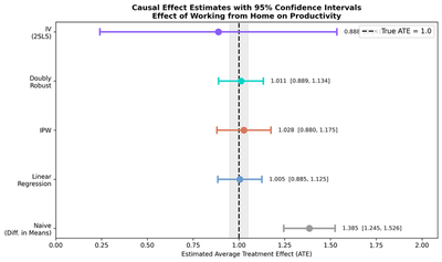
| Naive (Diff. in Means) | 1.3853 | 0.0716 | [1.245, 1.526] | 0.281 | No | None (biased) |
| Linear Regression | 1.0051 | 0.0614 | [0.885, 1.126] | 0.241 | Yes | Backdoor |
| IPW | 1.0275 | 0.0754 | [0.880, 1.175] | 0.296 | Yes | Backdoor |
| Doubly Robust (AIPW) | 1.0115 | 0.0623 | [0.889, 1.134] | 0.244 | Yes | Backdoor |
| IV (2SLS) | 0.8881 | 0.3303 | [0.241, 1.536] | 1.295 | Yes | Instrument |
All four causal methods recover the true ATE far better than the naive estimate. The backdoor methods (Regression, IPW, DR) are more precise because they use more information (the confounders directly), while IV is noisier but does not require observing all confounders. Crucially, the naive CI does not contain the true ATE — it is not just wrong, it is confidently wrong.
Uncertainty and precision: why standard errors matter
A point estimate without a standard error is like a weather forecast without a confidence range — it tells you the best guess but nothing about how much to trust it. In causal inference, standard errors (and the confidence intervals built from them) quantify the precision of our estimates: how much would the estimate change if we drew a different sample?
Why robust standard errors?
All standard errors in this analysis are robust (heteroskedasticity-consistent). Standard (“classical”) SEs assume that the variance of the outcome is the same for all observations. But in practice, productivity might be more variable for WFH workers than for office workers, or more variable for introverts than for extroverts. Robust SEs — specifically HC1 (White) standard errors for regression and IV, and influence-function SEs for IPW and DR — remain valid regardless of such differences. In observational studies, robust SEs should be the default.
How each method computes its standard error
| Method | SE Type | Intuition |
|---|---|---|
| Naive | Welch SE | Allows different variances in each group — like a two-sample t-test that does not assume equal variances |
| Linear Regression | HC1 (White) | The “sandwich” estimator wraps each observation’s squared residual in the variance formula, so large residuals for some observations do not distort the overall SE |
| IPW | Influence function | Each observation’s “influence” on the ATE is computed from the Hajek weighting formula; the variance of these individual influences gives the SE |
| Doubly Robust | Influence function | Same idea as IPW, but the influence function now includes both the outcome model and propensity score corrections, yielding a smaller SE |
| IV (2SLS) | Delta method + HC1 | Because IV divides the reduced-form by the first-stage, uncertainty in both stages propagates into the final SE via the delta method |
Comparing standard errors across methods
Method                     Robust SE  Relative to Regression
------------------------------------------------------------
Naive                         0.0716            1.17x
Linear Regression             0.0614            1.00x (reference)
IPW                           0.0754            1.23x
Doubly Robust                 0.0623            1.01x
IV (2SLS)                     0.3303            5.38x
Several patterns stand out:
Regression has the smallest SE (0.0614) because it directly models the outcome as a function of treatment and confounders. When the model is correctly specified (as in our simulation), this is the most efficient approach.
DR is nearly as precise (0.0623) because it too uses the outcome model, supplemented by propensity score corrections. When both models are correct, DR achieves the semiparametric efficiency bound.
IPW is slightly less precise (0.0754, 1.23x) because it ignores the outcome model entirely. It only uses propensity scores to reweight observations. Think of it as throwing away useful information about the outcome-covariate relationship, which costs some precision.
IV is dramatically less precise (0.3303, 5.38x). This is the bias-variance tradeoff in action. IV does not condition on confounders — it uses only the exogenous variation provided by the instrument. Because the instrument (subway disruption) explains only 22% more WFH participation (first-stage coefficient = 0.219), the IV estimator must “amplify” a small signal, which amplifies noise too. The price of not needing to observe confounders is a much wider confidence interval.
The naive SE (0.0716) is small but misleading. The naive estimate is precise (narrow CI) but wrong — its CI does not even contain the true ATE. This illustrates a critical lesson: a small standard error does not mean a good estimate. Precision without validity is worthless. The naive estimate is precisely estimating the wrong thing (a confounded association rather than a causal effect).
Step 4: Refute — Test robustness
The final step in DoWhy is refutation — a set of automated tests that check whether the estimate is robust to various challenges.
Placebo treatment test
Randomly permute the treatment variable so that no real causal effect exists. If our method is working correctly, the estimated effect should collapse to zero.
refute_placebo = model_backdoor.refute_estimate(
    estimand_backdoor,
    estimate_reg_bd,
    method_name="placebo_treatment_refuter",
    placebo_type="permute",
    num_simulations=100,
)
Refute: Use a Placebo Treatment
Estimated effect: 1.005
New effect: -0.00003
p value: 0.96
The placebo effect is essentially zero (-0.00003), confirming that the original effect is not an artifact. If the placebo test had returned a large effect, it would suggest that our model is picking up spurious patterns rather than genuine causal relationships.
Random common cause test
Add a randomly generated variable as an additional confounder. If the estimate is robust, it should not change.
refute_random = model_backdoor.refute_estimate(
    estimand_backdoor,
    estimate_reg_bd,
    method_name="random_common_cause",
    num_simulations=100,
)
Refute: Add a random common cause
Estimated effect: 1.005
New effect: 1.005
p value: 0.98
The estimate remains unchanged at 1.005 after adding a random confounder (p = 0.98). This confirms that our estimate is not fragile — it does not shift when irrelevant variables are added.
Data subset test
Re-estimate on a random 80% subsample of the data. A robust estimate should be stable across subsamples.
refute_subset = model_backdoor.refute_estimate(
    estimand_backdoor,
    estimate_reg_bd,
    method_name="data_subset_refuter",
    subset_fraction=0.8,
    num_simulations=100,
)
Refute: Use a subset of data
Estimated effect: 1.005
New effect: 0.999
p value: 0.64
The subsample estimate of 0.999 is nearly identical to the full-sample estimate of 1.005 (p = 0.64), confirming stability.
Two identification strategies: a comparison
This tutorial introduced two fundamentally different approaches to causal identification. Understanding when each applies is essential for choosing the right method in practice.
Selection on observables (backdoor criterion)
When to use: You believe you have measured all variables that simultaneously cause treatment and outcome.
Assumption: Unconfoundedness — conditional on observed confounders, treatment assignment is “as good as random.”
Methods: Linear Regression, IPW, Doubly Robust
Strength: More precise estimates (lower variance) because you use confounder information directly.
Weakness: If you miss even one confounder, the estimate is biased. There is no way to test the unconfoundedness assumption from data alone.
Instrumental variables
When to use: You have a variable that affects treatment but not the outcome directly, and you suspect unmeasured confounders.
Assumptions: Relevance (instrument affects treatment), exclusion restriction (instrument does not directly affect outcome), independence (instrument is not caused by confounders).
Method: IV / 2SLS
Strength: Valid even with unmeasured confounders.
Weakness: Noisier estimates (higher variance). The exclusion restriction cannot be tested from data — it must be justified by domain knowledge.
Takeaways
Naive comparisons are misleading when confounders are present. The naive estimate of 1.39 was 39% too high because introverts self-selected into WFH. Its narrow CI [1.25, 1.53] does not even contain the true ATE — a case of being precisely wrong.
Selection on observables (backdoor criterion) works when you have measured all confounders. Three methods — regression, IPW, and doubly robust — all recovered the true ATE within 3%, with robust SEs between 0.061 and 0.075.
Instrumental variables provide a different identification strategy that works even with unmeasured confounders, at the cost of a 5x larger standard error (0.33 vs 0.06).
Doubly robust estimation offers the best of both worlds: insurance against misspecification and near-optimal precision (SE = 0.062, nearly matching regression).
Standard errors measure precision, not validity. The naive estimate has a small SE but is biased. IV has a large SE but is unbiased under weaker assumptions. Always consider both bias and variance when choosing a method.
Robust standard errors (HC1, influence function) should be the default in observational studies. They remain valid even when error variances differ across groups.
DoWhy’s four-step framework forces transparency: declare your assumptions (Model), verify identifiability (Identify), compute the effect (Estimate), and test robustness (Refute).
Simulated data with known truth is the best way to learn causal inference — you can verify that methods work before applying them to real data where the answer is unknown.
Exercises
Break the exclusion restriction. Modify the DGP so that
subway_disruptiondirectly affectsproductivity(e.g., add+ 0.5 * subway_disruptionto the outcome equation). Re-run the IV estimate. Does it still recover the true ATE?Add an unmeasured confounder. Add a new variable
self_disciplinethat affects bothwork_from_homeandproductivity, but do NOT include it inCONFOUNDERS. Compare how the backdoor methods (now biased) and IV (still valid) perform.Try a nonlinear DGP. Replace the linear productivity equation with a nonlinear one (e.g., add an interaction term
0.3 * introversion * work_from_home). Does linear regression still work well? What about the doubly robust estimator?
References
- Sharma, A., & Kiciman, E. (2020). DoWhy: An end-to-end library for causal inference. arXiv preprint arXiv:2011.04216.
- Pearl, J. (2009). Causality: Models, Reasoning, and Inference (2nd ed.). Cambridge University Press.
- Angrist, J. D., & Pischke, J. S. (2009). Mostly Harmless Econometrics. Princeton University Press.
- Rosenbaum, P. R., & Rubin, D. B. (1983). The central role of the propensity score in observational studies for causal effects. Biometrika, 70(1), 41–55.
- Robins, J. M., Rotnitzky, A., & Zhao, L. P. (1994). Estimation of regression coefficients when some regressors are not always observed. Journal of the American Statistical Association, 89(427), 846–866.
Carlos Mendez
Associate Professor of Development Economics
My research interests focus on the integration of development economics, spatial data science, and econometrics to better understand and inform the process of sustainable development across regions.