Causal Machine Learning and the Resource Curse

Heterogeneous treatment effects with EconML’s CausalForestDML

0.240DML mining ATE · true 0.250

−0.141naive bias removed

0.089GATE range · institutions moderate

Carlos Mendez

Nagoya University (GSID)

June 11, 2026

The Tension

Act I

Is resource wealth a blessing or a curse? The honest answer is: it depends on whom you ask

A district strikes a mine. Nighttime lights climb. But the district next door — same mineral, weaker institutions — barely flickers.

One average effect cannot describe both. The question is not “what is the effect of mining?” but for whom, and how much?

The resource-curse literature argues the answer hinges on local institutional quality. A single ATE collapses that variation. We want the effect as a function of district characteristics, not one headline number.

The naive comparison says mining barely helps — and it is wrong by 56%

Contrast	Naive	Truth	Bias
Mining vs none (1-0)	0.109	0.250	−0.141
High vs low price (3-1)	0.413	0.300	+0.113

Mining districts differ systematically — worse geography, weaker institutions — so a raw difference-in-means confounds selection with effect.

The naive 1-0 estimate of 0.109 is a 56% underestimate of the true 0.250. Mining districts have characteristics that independently depress development, biasing the simple comparison downward. This is the bias the causal forest must remove.

We want the CATE — a function of \(\mathbf{x}\), not a single number

\[\tau(\mathbf{x}) = E\{Y_i(1) - Y_i(0) \mid \mathbf{X}_i = \mathbf{x}\}\]

Where \(\tau(\cdot)\) bends with \(\mathbf{x}\), mining helps some districts more than others — that bend is the whole point.

Estimand: the Conditional Average Treatment Effect. Read it as: among districts that look like x, what is the average gap between the treated and untreated potential outcomes? When τ is constant in x, one ATE summarizes everything. When it bends, we have heterogeneity. The causal forest estimates that bend without us pre-specifying its shape.

Where we’re going

• The lab: a simulated 300-district panel with known ground truth
• Double Machine Learning — residualize away the confounders
• The causal forest recovers the ATE and discovers the price non-linearity
• GATEs reveal that institutions moderate mining, but not price

The Investigation

Act II

A simulated lab where we know the right answers in advance

• 3,000 district-years — 300 districts, 8 countries, 2003–2012
• Outcome — log nighttime lights (a proxy for development)
• Treatment — four levels: no mining, then low / medium / high mineral prices
• Ground truth built in — so we can check the method recovers it

Structure mirrors Hodler, Lechner & Raschky (2023); because we built the data, the identifying assumption holds by construction.

Using simulated data with known parameters is the trick: we can verify the forest recovers the true ATEs. The DGP follows a real study so the structure is realistic, but the controlled setting lets us validate the methodology rather than debate the economics.

The treatment is brutally imbalanced — 85% of district-years never mine

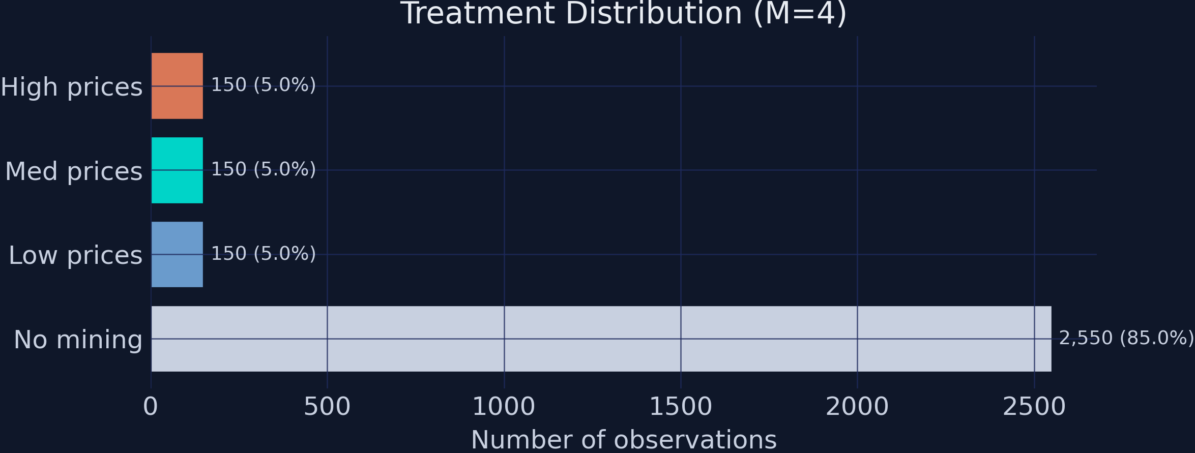
Treatment distribution. 2,550 control observations but only 150 per mining level — within-mining contrasts lean on just 300 rows.

The 85/5/5/5 split is what makes this hard. Plenty of controls, scarce treated units. Price-effect standard errors will be large because only 150 observations per level contribute, and within-mining comparisons (like 3-1) draw on 300.

DML residualizes both sides, then lets a forest read the remainder

\[Y_i = \tau(\mathbf{X}_i)\, T_i + g_0(\mathbf{X}_i, \mathbf{W}_i) + \varepsilon_i\]

\[T_i = m_0(\mathbf{X}_i, \mathbf{W}_i) + v_i\]

Subtract the predictable parts: \(\tilde Y_i = \tau(\mathbf{X}_i)\,\tilde T_i + \varepsilon_i\). The nuisance functions \(g_0, m_0\) exist only to be subtracted out.

Partially linear model (Robinson 1988; Chernozhukov et al. 2018). Estimate g0 and m0 with any flexible learner, residualize Y and T, then regress Y-tilde on T-tilde with a covariate-dependent slope. That slope is the CATE. This is Frisch-Waugh-Lovell with machine-learning residualizers.

Why first-stage errors barely matter: Neyman orthogonality

\[\left.\frac{\partial}{\partial \eta} E[\psi(W; \tau, \eta)] \right|_{\eta = \eta_0} = 0\]

At the truth, the estimating equation is flat in the nuisances. A 10% error in \(\hat g_0\) enters \(\hat\tau\) at order \((0.10)^2 \approx 0.01\) — second order.

This is the self-righting-boat property. Even if Gradient Boosting converges at the slow O(n^-1/4) rate, the second-stage estimate of tau stays root-n-consistent and asymptotically normal. A naive plug-in two-stage procedure loses this and inherits the slow nuisance rate.

Configure CausalForestDML: honest trees, cross-fitting, grouped by district

est_ntl = CausalForestDML(
    model_y=GradientBoostingRegressor(n_estimators=200, max_depth=4),
    model_t=GradientBoostingClassifier(n_estimators=200, max_depth=4),
    discrete_treatment=True, categories=[0, 1, 2, 3],
    n_estimators=500, min_samples_leaf=10,
    honest=True,       # split-chooser ≠ leaf-estimator → valid CIs
    inference=True,    # Bootstrap-of-Little-Bags standard errors
    cv=5,              # 5-fold cross-fitting
)
est_ntl.fit(Y, T, X=X, W=W,
            groups=df['district_id'].values)  # GroupKFold: no district leakage

honest=True separates the sample that chooses splits from the one that estimates leaf means — that licenses valid confidence intervals. cv=5 cross-fits the nuisances. groups=district_id triggers GroupKFold so a district never straddles folds, blocking first-stage leakage. Note: GroupKFold is NOT clustered SEs — BLB still treats observations as independent.

Identification rests on one untestable assumption — not on the algorithm

\[\{Y_i(0), Y_i(1), Y_i(2), Y_i(3)\} \perp T_i \mid (\mathbf{X}_i, \mathbf{W}_i)\]

Conditional Independence: once we know a district’s geography, institutions, country, and year, mining status is as good as random. We built the data, so it holds here — in real data it is untestable.

The CIA, a.k.a. unconfoundedness or selection on observables. Two real-world violation channels: mineral surveys that predict both mining and unrelated infrastructure, and political connections that attract both concessions and roads. “We used a causal forest” does not relax the CIA — the method is only as credible as the controls.

The Resolution

Act III

The forest recovers a mining ATE of 0.240 — within sampling error of the true 0.250

0.240

mining-vs-none ATE (1-0), SE 0.070, 90% CI [0.124, 0.355] · true value 0.250

Finding 1. The naive difference was 0.109; DML lifts it to 0.240, eliminating nearly all of the −0.141 bias. Because the outcome is log NTL, 0.24 ≈ a 27% rise in unlogged lights. All three mining-vs-none contrasts are positive and well separated from zero.

DML removes the −0.141 confounding bias the naive estimator carried

−0.141

bias in the naive 1-0 estimate (0.109 vs truth 0.250) · the forest erases almost all of it

The headline pedagogical point: residualizing against observed confounders is what closes the gap. The selection bias came from mining districts’ systematically worse geography and institutions; conditioning on (X, W) neutralizes it.

The forest discovers a non-linear price gradient — without being told to look

Contrast	ATE	SE	Sig.?
Medium vs low (2-1)	0.029	0.101	no
High vs low (3-1)	0.220	0.101	5%
High vs medium (3-2)	0.191	0.109	10%

Flat from low to medium, then a jump at high prices — shape discovery with no functional form pre-specified.

Finding 2. The 2-1 interval [−0.137, 0.194] easily contains zero: medium prices add nothing detectable beyond basic mining. 3-1 is significant at 5%. The forest recovered the true price-response curve’s qualitative shape — this is what causal ML buys you over a parametric interaction.

Institutions amplify the mining effect — stronger constraints, larger payoff

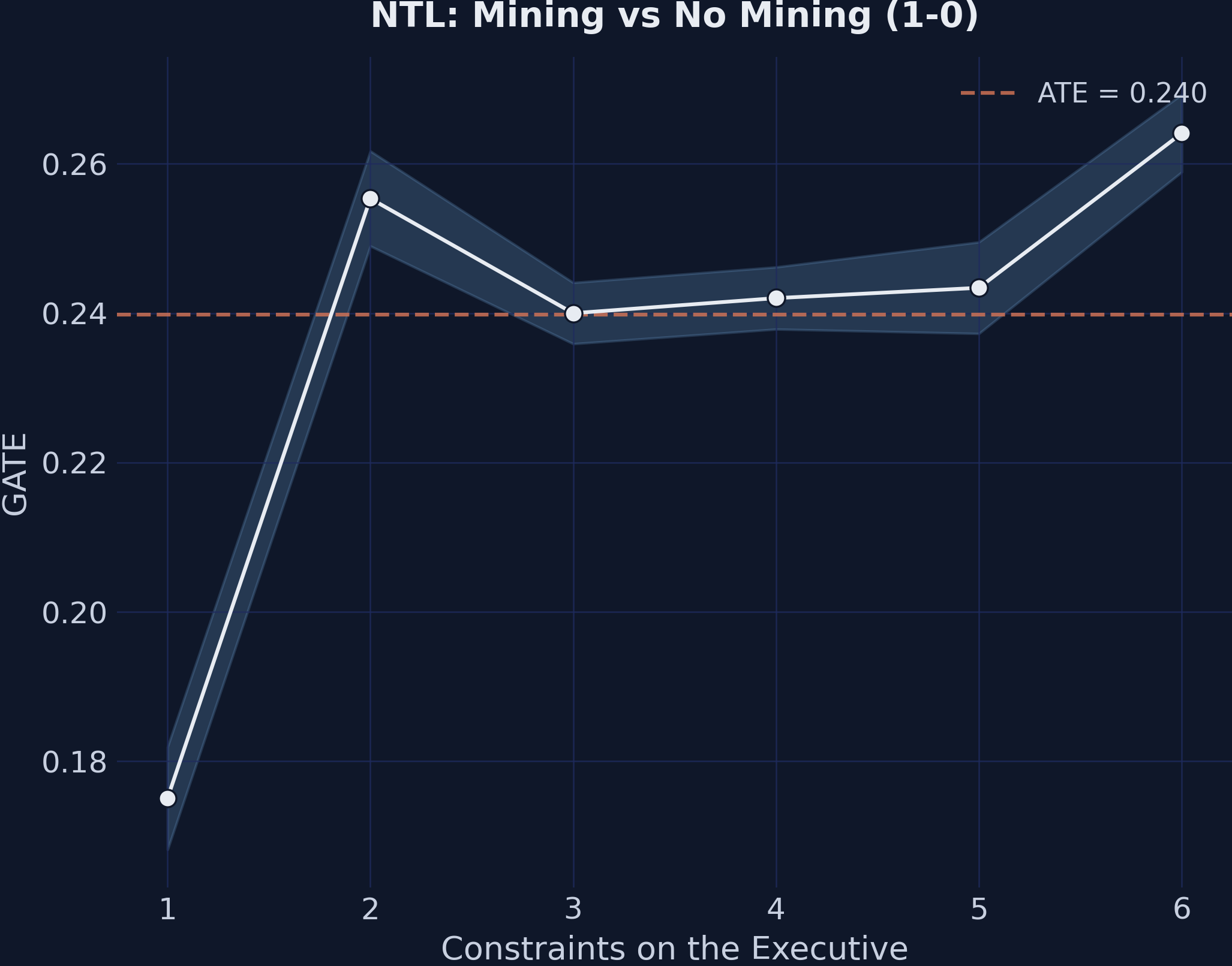
GATEs for the mining effect (1-0) by executive constraints. The upward slope: stronger institutions amplify the economic benefit of mining.

Finding 3a. The mining-effect GATE climbs roughly monotonically from 0.175 at the weakest institutions to 0.264 at the strongest — a range of 0.089. Substantively: weak institutions cut the development gain from mining roughly in half. This is the structural prediction of Mehlum-Moene-Torvik.

The price effect is flat across institutions — a non-finding that is the finding

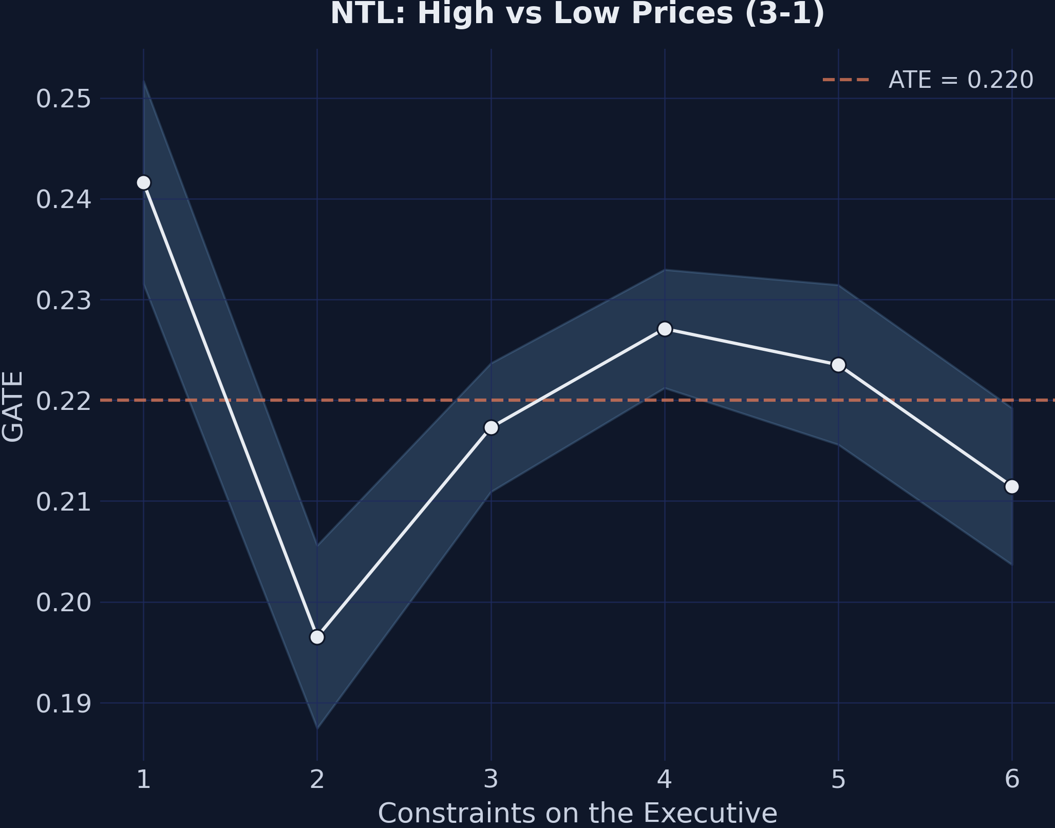
GATEs for the price effect (3-1) by executive constraints. The flat line: institutions do not moderate price effects (range 0.045).

Finding 3b. The price-effect GATE spans only 0.045 with no monotone pattern. By construction the price step is uniform across institutional environments, so the forest correctly flat-lines. The asymmetry — institutions shaping the mining margin but not the price margin — is exactly what a flexible τ(x) can discover and a single interaction term would miss.

A second institutional measure cross-validates the same asymmetry

Mining effect (1-0)

• rises with quality of government
• matches the exec.-constraints range of 0.089
• institutions amplify mining

Price effect (3-1)

• flat across quality of government
• matches the exec.-constraints range of 0.045
• institutions do not touch price

Quality of government tells the same story as executive constraints — robust to the institutional measure.

The GATEs-by-quality-of-government plots reproduce the pattern: mining effect positively sloped, price effect flat. Two different institutional proxies, one conclusion — the moderation is in mining, not price.

Beware: the most “important” features are not the moderators

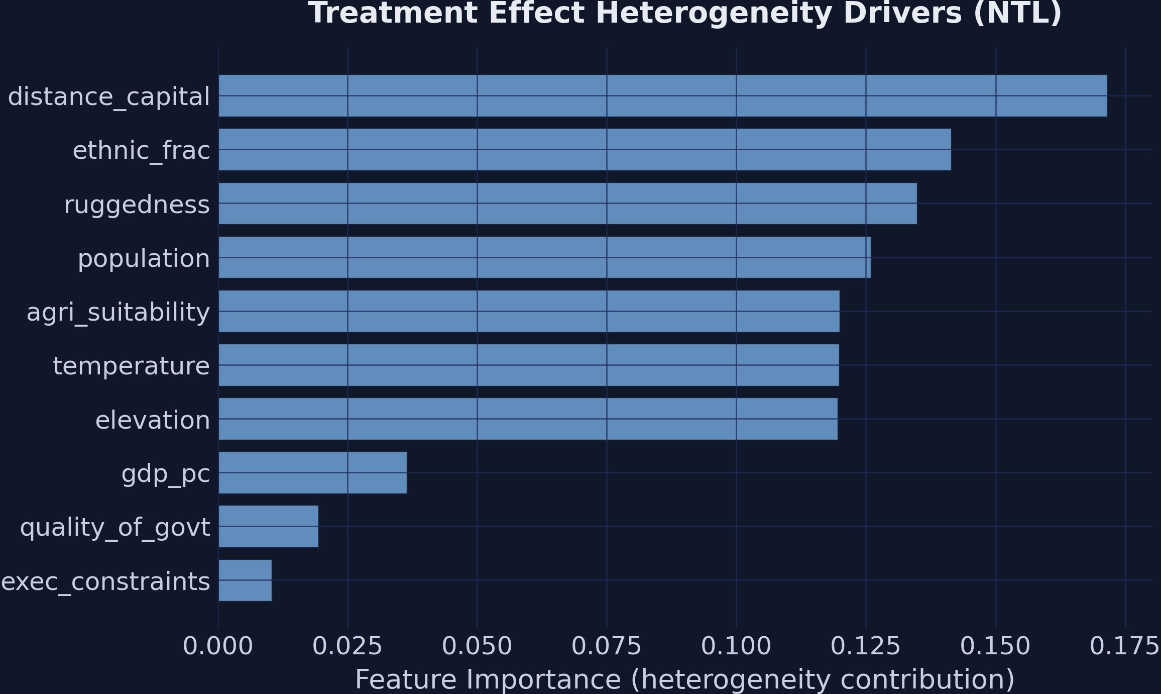
Feature importance for heterogeneity. Geographic variables dominate split frequency, yet institutions are the true moderators.

exec_constraints is dead last by importance (0.014) yet it is what bends the mining effect. Importance counts variance-weighted split frequency; continuous variables (distance_capital, ethnic_frac) offer many thresholds and get picked often. Coarse discrete moderators with 6 levels accumulate little importance even when one split carries the heterogeneity. Read importance as screening, confirm with GATEs.

A depth-2 tree turns the forest’s heterogeneity into a story you can tell aloud

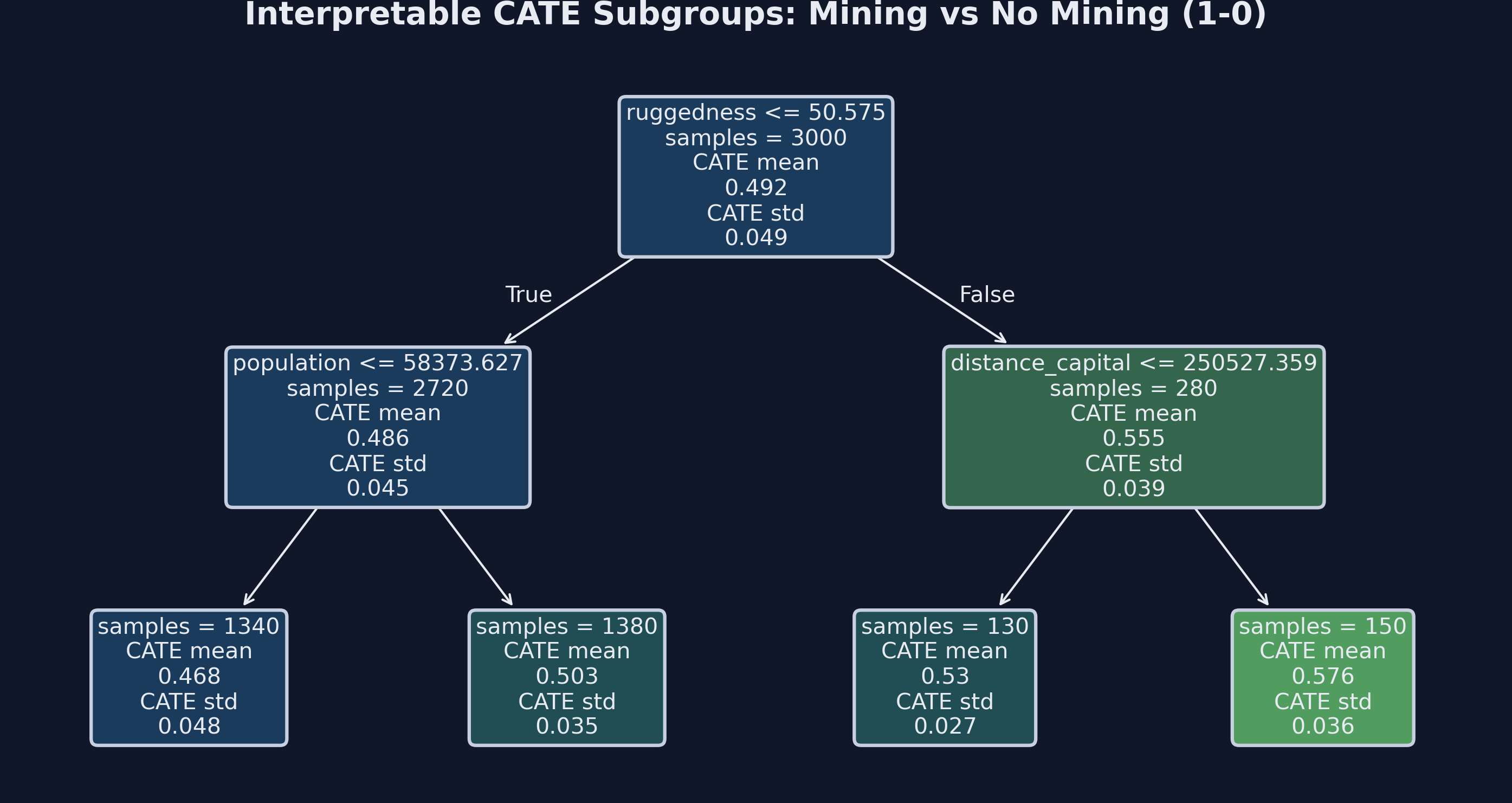
Depth-2 CATE interpreter for the mining effect. Each leaf reports the mean estimated CATE for the subgroup defined by the splits above it.

SingleTreeCateInterpreter fits a shallow tree to the predicted CATEs themselves — a summary of the heterogeneity surface, not a re-estimation. GATEs are hypothesis-driven (you name the moderator); the interpreter is exploratory (it finds the best splits). Run both: GATEs test theory, the interpreter audits it.

The strongest objection — and the answer

Objection. A machine that picks controls cannot manufacture causal identification.

Response. Exactly right. \(\tau(\mathbf{x})\) is identified only under the Conditional Independence Assumption — the forest earns honest intervals, but it cannot rule out an unobserved confounder.

Steelman the critique. The forest discovers heterogeneity flexibly and earns honest confidence intervals, but it cannot relax the identifying assumption. With real data the CIA is untestable; here it holds only because we built it in. DML disciplines estimation and inference; it does not relax identification. BLB SEs even treat panel observations as independent, so true clustered SEs would be larger. The Stata companion uses vce(cluster district_id). The method is a tool for credible heterogeneity estimation, conditional on identification holding.

Let the data reveal for whom — but never forget the assumption that makes it causal.

The single takeaway. Causal forests recover the average, discover non-linear shape, and surface institutional moderation without parametric pre-specification — and they remain exactly as credible as the conditional independence assumption underneath them.