Do Institutions Cause Prosperity?

An IV tutorial: instrumenting modern institutions with settler mortality

0.9442SLS effect of institutions

+81%larger than naive OLS

64ex-colonies, one instrument

Carlos Mendez

Nagoya University (GSID)

June 11, 2026

The Tension

Act I

Richer countries have better institutions — but a correlation cannot tell us which way the arrow points

Stronger property-rights institutions track far higher income across countries. The gradient is real and huge.

But maybe rich countries simply afford better courts — or geography drives both. The slope is correlation; it cannot prove cause.

This is the central problem of the whole tutorial. Everyone agrees something about institutions matters, but the simple cross-country plot is contaminated by reverse causality, omitted variables, and measurement error. We need a research design, not just a regression.

Across every specification, the causal effect lives near 0.9 — well above the OLS slope of 0.5

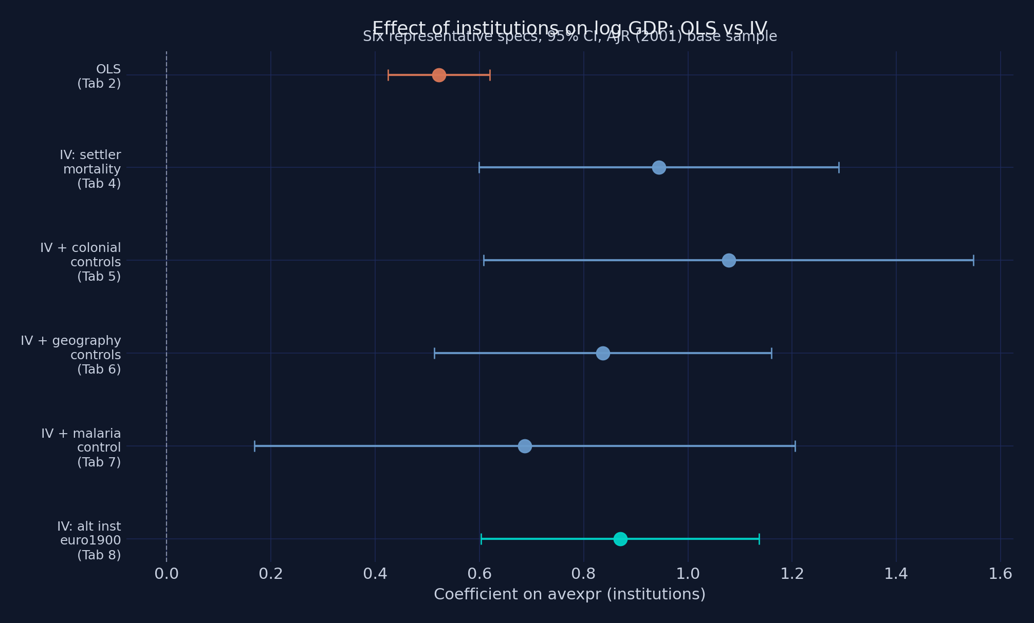
Coefficient on institutions (\(\hat\beta\)) across six specifications, 95% CIs. Orange = naive OLS; steel = IV with settler mortality; teal = an alternative instrument.

Spoiler figure. Don’t explain every bar yet — just plant that the OLS estimate (orange, 0.522) sits well below every IV variant (0.7–0.94). We earn each one in Act II and return to this picture at the end.

Where we’re going

• Why OLS is biased here — reverse causality, omitted variables, measurement error
• The three conditions every instrument must satisfy
• Settler mortality as the instrument: first stage and reduced form
• 2SLS as a single ratio — and what the 0.944 number really is

The Investigation

Act II

Institutions are endogenous, so OLS does not estimate the causal effect

• Reverse causality — rich countries can afford better institutions
• Omitted variables — geography, culture, human capital drive both
• Measurement error — the institutions index is a noisy proxy, attenuating OLS

A regressor is endogenous when it correlates with the error term; then OLS is biased even with infinite data.

Use the bathroom-scale analogy: standing on a scale while holding a weight gives a real reading, but it bundles your body weight with the weight you hold. OLS bundles the causal effect with confounding. We need a different tool to separate them.

The structural model: the error is correlated with the regressor — that is the whole problem

\[Y_i = \alpha + \beta X_i + U_i, \qquad \mathrm{Cov}(X_i, U_i) \neq 0\]

The outcome \(Y_i\) (log GDP) depends on the endogenous regressor \(X_i\) (institutions) plus an error \(U_i\) that gathers every unobserved driver of income.

The target is \(\beta\), the true causal coefficient. The non-zero \(\mathrm{Cov}(X_i, U_i)\) is exactly why OLS misses it.

U collects geography, culture, human capital, and measurement noise — everything we cannot model explicitly. IV will replace X with only the part of it that an external instrument predicts.

A valid instrument must clear three bars: relevance, exclusion, exogeneity

What an instrument \(Z\) must do

• Relevance — \(Z\) moves \(X\) (testable: first-stage \(F\))
• Exclusion — \(Z\) affects \(Y\) only through \(X\)
• Exogeneity — \(Z\) is uncorrelated with \(U\)

AJR’s instrument

• \(Z =\) log settler mortality circa 1700
• Deadly colonies became extractive; safe colonies got European-style institutions
• 1700 mortality cannot react to 1995 GDP

Relevance is the only one we can test directly. Exclusion and exogeneity are AJR’s substantive claim — that settler mortality affects modern income only through the institutions it shaped. Picture a coin flip deciding who gets a drug: it changes outcomes only through whether the patient takes the drug.

The lab: AJR’s base sample of 64 ex-colonies, one instrument, a 60-fold income range

• Outcome — log GDP per capita 1995 (logpgp95), spanning roughly $450 to $27,400
• Endogenous regressor — protection from expropriation (avexpr), 0–10
• Instrument — log settler mortality (logem4), nearly six log points of spread

The baseco==1 subset of the wider ~163-country world: 64 ex-colonies with valid mortality data.

Restricting to ex-colonies lowers mean institutions from 6.99 to 6.52 and the European-settler share from 30% to 16%. Australia, New Zealand, and the US sit at the low-mortality, strong-institution corner; Sierra Leone, Niger, and Mali at the high-mortality, weak-institution corner.

Relevance holds: a one-log-point rise in mortality cuts institutions by 0.607, F = 16.85

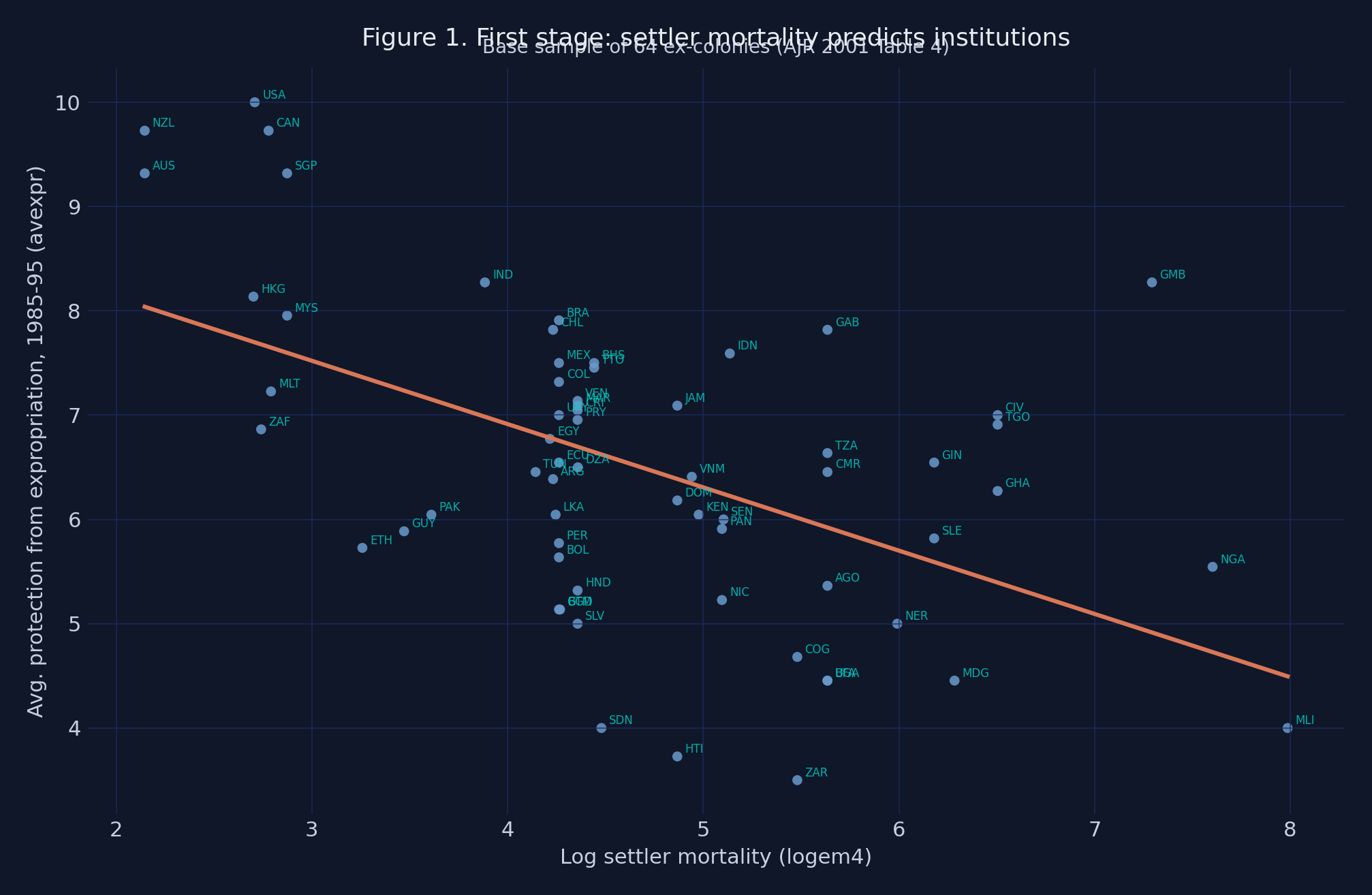
First-stage scatter of institutions (avexpr) on log settler mortality (logem4), 64 ex-colonies. Slope \(-0.607\), \(F = 16.85\), \(R^2 = 0.27\).

The first-stage F of 16.85 is just above the Staiger-Stock rule of thumb of 10 and almost exactly at the Stock-Yogo iid threshold of 16.38. Honest disclosure: this is borderline-strong, not comfortable — several robustness specs push F below 5, where the confidence intervals should not be taken literally.

The reduced form confirms it: deadlier colonies are about 30 times poorer today

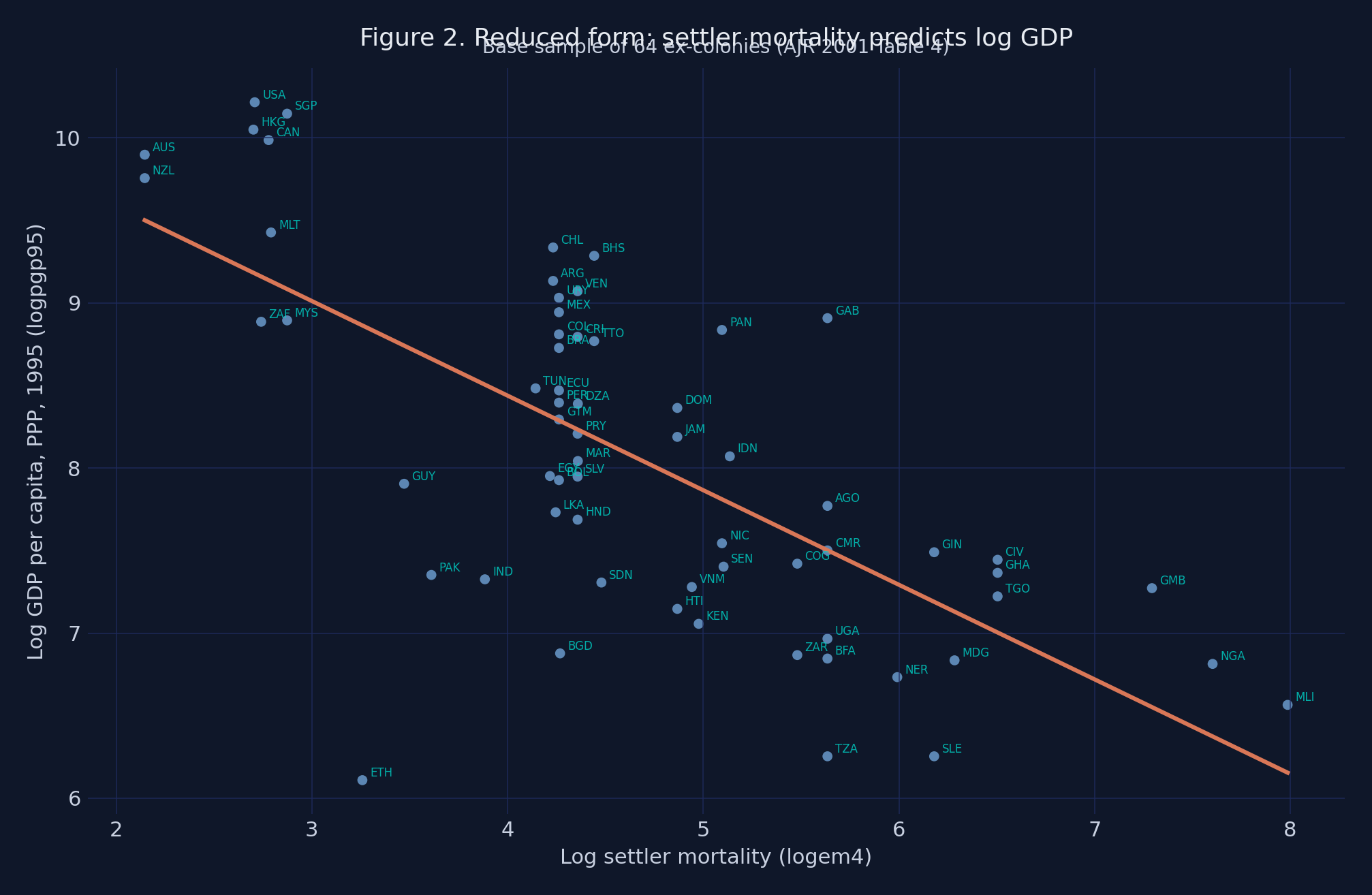
Reduced-form scatter of log GDP (logpgp95) on log settler mortality (logem4). The slope (\(\approx -0.573\)) is the total effect of the instrument on the outcome.

Across the 5.8-log-point span of mortality, the fitted line predicts a GDP gap of about 3.4 log points — roughly 30 times poorer for the deadliest colonies. This total effect is what 2SLS decomposes into the first-stage and second-stage channels.

2SLS is just one division: the reduced-form slope over the first-stage slope

\[\hat\beta_{2SLS} = \frac{\widehat{\mathrm{Cov}}(Y, Z)}{\widehat{\mathrm{Cov}}(X, Z)} = \frac{\hat\beta_{RF}}{\hat\beta_{FS}} = \frac{-0.573}{-0.607} = 0.944\]

The numerator is the total effect of the instrument on the outcome; the denominator rescales by how much the instrument moves institutions.

The whole IV machinery, in one ratio: \(-0.573 / -0.607 = 0.944\).

The rope analogy: if pulling a rope by 1 meter moves a hidden box by 0.6 meters and lifts a flag by 0.57 meters, then moving the box by 1 meter lifts the flag by 0.57/0.6 = 0.94. IV is this proportion calculation.

Two libraries, one formula: pyfixest gives the estimate, linearmodels the diagnostics

import pyfixest as pf
from linearmodels.iv import IV2SLS
# structural 2SLS via pyfixest's "exog | endog ~ instrument" syntax
m_iv = pf.feols("logpgp95 ~ 1 | avexpr ~ logem4", data=base, vcov="HC1")
# weak-IV F, Wu-Hausman, Hansen J — the tests pyfixest does not report
res  = IV2SLS(base["logpgp95"], X_exog, base[["avexpr"]], base[["logem4"]]).fit(cov_type="robust")

pyfixest excels at the idiomatic formula syntax and the structural estimate; linearmodels supplies the Kleibergen-Paap-style first-stage F, the Wu-Hausman endogeneity test, and the Hansen J overidentification test. Each does the job it does best. Both agree on the point estimate to six decimals.

Naive OLS sees only half the story: a slope of 0.522

0.522

OLS estimate of \(\hat\beta\) on institutions, base sample (SE 0.050) — the benchmark IV will overturn

0.522 in the 64-country base sample, stable across specifications and significant at the 1% level. But it carries reverse causality, omitted-variable bias, and attenuation from measurement error. The question is how much of the 0.522 is bias.

The strongest objection — and the answer

Objection. Maybe the tropical disease environment that killed settlers still depresses productivity today — a direct arrow from mortality to GDP that breaks the exclusion restriction.

Response. Adding modern health controls pulls \(\hat\beta\) down only to 0.55–0.69 — still above OLS — and the overidentification tests (Hansen J, \(p\) = 0.18–0.79) do not reject joint exogeneity. The threat is real but bounded; it does not erase the effect.

Steelman, don’t strawman. Health is the tightest empirical challenge. AJR read modern health as a “bad control” downstream of institutions; a critic reads it as genuine exogenous variation. The data alone cannot adjudicate, but the coefficient survives — it never collapses to zero.

The Resolution

Act III

Instrumenting institutions recovers a causal effect of 0.944 — Wu-Hausman confirms OLS was biased

0.944

2SLS \(\hat\beta\) on institutions (SE 0.176, 95% CI [0.60, 1.29]); Wu-Hausman \(F = 24.22\), \(p < 0.0001\)

The Wu-Hausman test rejects the null that OLS is consistent — the IV–OLS gap is statistical evidence of bias, so IV is empirically warranted, not just theoretically motivated. The point estimate matches the Stata ivreg2 reference to three decimals.

The causal effect is 81% larger than OLS — measurement error, not endogeneity, dominated the bias

Estimator	\(\hat\beta\)	SE	95% CI
OLS (base sample)	0.522	0.050	—
2SLS (settler mortality)	0.944	0.176	[0.60, 1.29]

IV > OLS by 81% implies attenuation from measurement error outweighed reverse causality and omitted variables.

Three biases pull in opposite directions: reverse causality and omitted variables push OLS up; classical measurement error in the institutions index pulls it down. IV landing 81% above OLS says the downward attenuation dominated — de-noising the proxy reveals a steeper causal slope, not a shallower one.

The 0.944 is a LATE for compliers, and it leans on assumptions only partly testable

What it is

• A Local Average Treatment Effect (Imbens-Angrist)
• The effect for complier countries near the colonization margin
• Not a population average for every country

What still carries weight

• Exclusion is untestable in principle
• Albouy (2012): ~36% of mortality data imputed or shared
• Hansen J cannot detect coordinated witnesses

2SLS recovers a complier effect, not the population ATE. Albouy’s imputation critique limits what overidentification non-rejection can buy — shared imputation noise would let the alternative instruments agree falsely. Honest IV reporting names both the estimand and the maintained assumptions.

Let the disease environment of 1700, not the regression of 1995, identify the effect of institutions.

The single takeaway. A credible instrument turns a contaminated 0.522 correlation into a 0.944 causal estimate — implying institutional reform is roughly twice as valuable as naive cross-country regressions suggest. The design, not the data, does the work.