Multiscale Geographically Weighted Regression

Spatially varying economic convergence across Indonesia’s 514 districts

0.762MGWR R² vs 0.214 global

44districts per local window

149 / 514significant catching-up (29%)

Carlos Mendez

Nagoya University (GSID)

June 11, 2026

The Tension

Act I

One national convergence number forces 514 different places onto a single line

A standard convergence test asks: do poorer regions catch up to richer ones? For Indonesia it answers with one coefficient: \(\beta = -0.195\).

But Indonesia spans 17,000 islands across 5,000 km of ocean. Should Sumatra and Papua really share the same catching-up rate?

This is the central tension of the post. A single global slope averages over enormous geographic diversity. The whole point of MGWR is to ask whether that average hides where catching-up actually happens — and the answer turns out to be yes.

The global fit is so weak it explains barely a fifth of growth

Global \(\beta\)-convergence regression: log GDP per capita 2010 vs growth 2010–2018. One orange OLS line through 514 districts.

Spoiler tension figure. The slope is negative and highly significant (p < 0.001), so convergence “exists on average.” But look at the scatter — the dispersion around the line is enormous. R² is only 0.214. That low explanatory power is the entire motivation for going local.

Where we’re going

• The data: 514 Indonesian districts, initial income and subsequent growth
• The problem: a single coefficient hides spatial heterogeneity
• The method: GWR, then MGWR — each variable at its own spatial scale
• The payoff: R² jumps from 0.214 to 0.762, and only 29% of districts truly converge

The Investigation

Act II

The lab: 514 districts, one outcome, one predictor, a 5,000-km archipelago

• Outcome \(g_i\) — GDP growth rate, 2010–2018 (mean 0.39, range \(-2.05\) to \(+2.06\))
• Predictor \(\ln(y_{i,2010})\) — log GDP per capita in 2010 (range 7.17 to 13.44)
• Geography — 514 districts across 17,000 islands, from dense Java to remote Papua

Cross-section from the QuaRCS repository; convergence means a negative slope on initial income.

The richest district (13.44) is roughly 690,000 dollars per capita — likely a resource-extraction enclave — and the poorest (7.17) about 1,300 dollars. That range, plus growth from severe contraction to rapid expansion, is exactly the variance a single line cannot capture.

The naked-eye maps already show geography is organized, not random

Two-panel choropleth: (a) log GDP per capita 2010 and (b) growth rate 2010–2018. Patterns cluster — they are not scattered.

Before fitting anything, map the two variables. Initial income is highest in Jakarta and resource-rich Kalimantan/Papua; lowest in eastern Nusa Tenggara and Maluku. Growth tells a different story — some of the poorest Papua and Sulawesi districts grew fastest. Because these patterns are geographically organized, a spatial model should outperform a global one.

\(\beta\)-convergence is one global slope on initial income

\[g_i = \alpha + \beta \cdot \ln(y_{i,2010}) + \varepsilon_i\]

A negative \(\beta\) means poorer districts grow faster — the gap shrinks. Here \(\beta = -0.195\), but it is a single number for the whole country.

This is the classic growth-economics test. The sign of beta is the whole question: negative means convergence. The limitation is structural — one alpha, one beta, no room for geography to matter.

GWR lets every district keep its own slope and intercept

\[g_i = \alpha(u_i, v_i) + \beta(u_i, v_i) \cdot \ln(y_{i,2010}) + \varepsilon_i\]

Now \(\alpha\) and \(\beta\) are functions of location \((u_i, v_i)\) — one regression per place.

A distance-decay kernel weights nearby districts more. A bandwidth \(h\) sets how many neighbours each local regression listens to. GWR fits one regression per location, weighted by spatial proximity. Small bandwidth = highly local and noisy; large bandwidth = smooth, approaching the global model. The coefficients become maps instead of single numbers. But standard GWR has one catch — addressed on the next slide.

GWR’s flaw: one bandwidth for all variables — MGWR removes it

GWR

• One bandwidth \(h\) for all coefficients
• Intercept and slope forced to vary at the same spatial scale

MGWR

• A separate bandwidth per variable
• Back-fitting cycles each variable, optimizing \(h\) while others are held fixed

The “multiscale” point: baseline conditions may vary over large regions while convergence speed shifts sharply between neighbours.

This is the methodological advance. MGWR relaxes GWR’s single-bandwidth constraint through iterative back-fitting, letting each variable find its own optimal spatial scale from the data. It assumes local stationarity — the relationship is approximately constant among the nearest h districts even if it differs across the full map.

Four lines fit MGWR on standardized variables in Python

y = gdf["g"].values.reshape((-1, 1)); X = gdf[["ln_gdppc2010"]].values
coords = list(zip(gdf["COORD_X"], gdf["COORD_Y"]))

Zy = (y - y.mean(0)) / y.std(0)          # standardize: required for MGWR
ZX = (X - X.mean(0)) / X.std(0)          # makes bandwidths comparable

selector = Sel_BW(coords, Zy, ZX, multi=True, spherical=True)
bw = selector.search()                    # back-fitting finds per-variable h
results = MGWR(coords, Zy, ZX, selector, spherical=True).fit()

Standardization is load-bearing — without it the per-variable bandwidths are not comparable. The spherical=True flag computes great-circle distances, essential across a 5,000-km archipelago. multi=True is what makes this MGWR rather than plain GWR.

MGWR picks a tight window of 44 districts — about 8.6% of the sample

Variable	Bandwidth	\(ENP_j\)	Adj. \(t(95\%)\)
Intercept	44	26.81	3.13
Convergence slope	44	25.27	3.11

Both variables converge on the same window here; with more covariates MGWR could assign each a very different scale.

A bandwidth of 44 out of 514 is highly local — each district’s regression listens only to its 44 nearest neighbours. That tight window is the signal that the convergence relationship genuinely varies across the archipelago rather than being a smooth national gradient.

The intercept reveals an east–west growth gradient

MGWR intercept map (bandwidth = 44). Western districts negative; eastern districts positive.

The intercept captures baseline growth after accounting for initial income. Western Indonesia — Sumatra and Java — grew less than the convergence model predicts. Eastern Indonesia — Papua, Maluku, Nusa Tenggara — grew more than expected. This likely reflects resource extraction, infrastructure investment, and fiscal transfers that boosted less-developed eastern regions in 2010–2018.

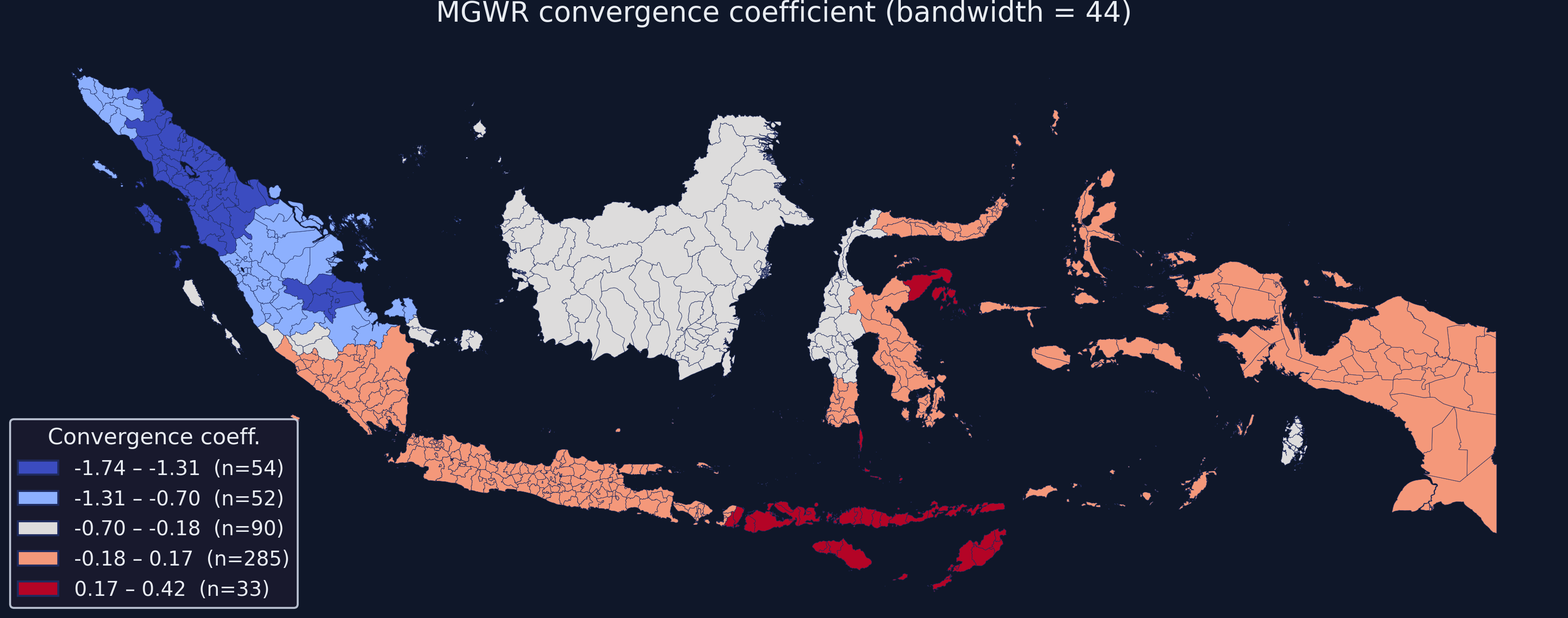
Catching-up is intense in western Sumatra, absent across most of the country

MGWR convergence-coefficient map. Deep blue (\(-1.74\)) = strong catching-up; light pink = no convergence.

This is the central finding. The single global beta of -0.195 hides a coefficient that ranges from -1.74 (strong local catching-up in western Sumatra and parts of Kalimantan) to +0.42 (localized divergence), with a median of -0.085 and a standard deviation of 0.553. Most of Java and eastern Indonesia sit near zero — the convergence relationship is essentially absent there.

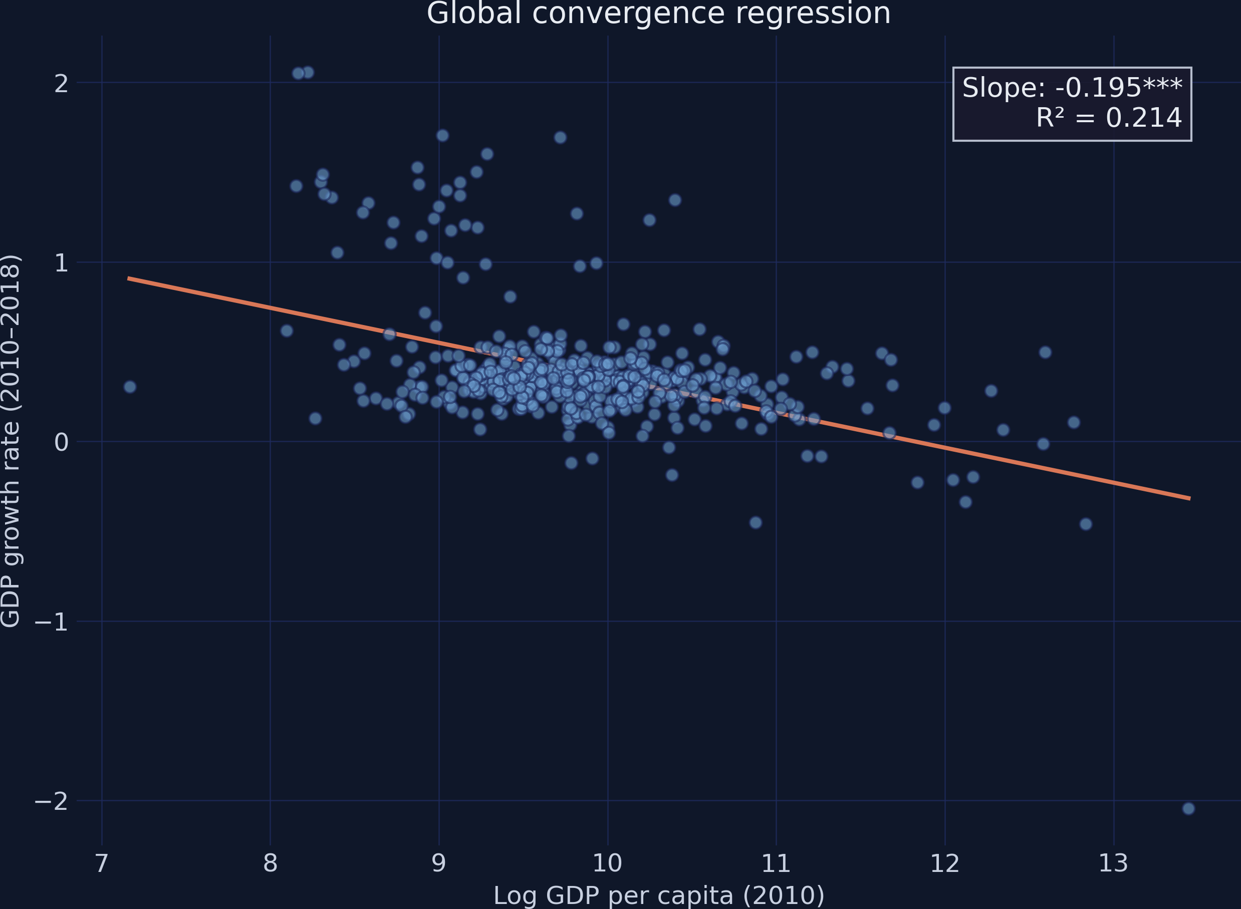
The local slope ranges from −1.74 to +0.42 — nowhere near a single −0.195

−1.74 → +0.42

range of the local convergence coefficient \(\hat\beta(u_i,v_i)\) · global OLS reports just \(-0.195\)

One giant number to make the heterogeneity visceral. The global model collapses this entire spread into a single point estimate. That collapse is precisely what MGWR recovers — and what a policymaker reading only the national number would never see.

The Resolution

Act III

Going local triples the explained variance and slashes AICc by 500

Metric	Global OLS	MGWR
\(R^2\)	0.214	0.762
Adj. \(R^2\)	0.212	0.736
AICc	1341.25	838.41
Bandwidth	all (514)	44

Adjusted \(R^2\) of 0.736 already nets out the 52 effective parameters — the gain is real, not overfitting.

R² more than triples, from 0.214 to 0.762. The AICc drop of over 500 is decisive — a difference that large is not explainable by extra flexibility alone. The effective parameter count is 52.1, far more than OLS’s 2 but far less than fitting 514 separate regressions (1,028 parameters). MGWR finds the right complexity automatically.

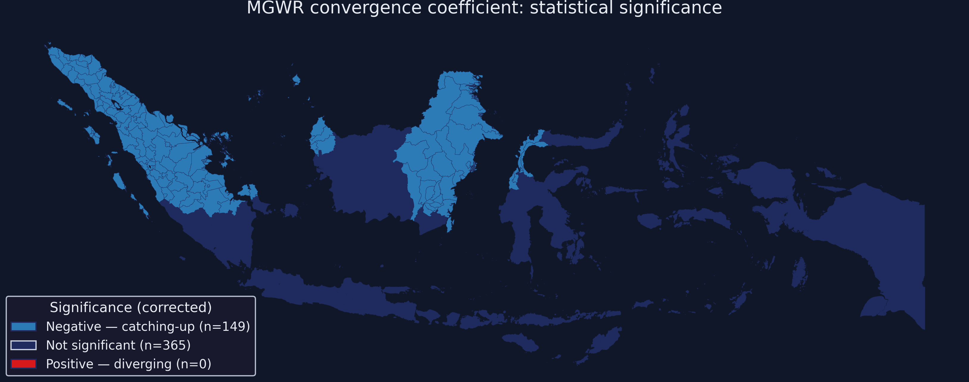
Only 149 of 514 districts truly converge — and none diverge

Significance map: blue = significant catching-up (149 districts), grey = not significant (365), no significant divergence.

After correcting for multiple testing, 149 districts (29%) show significant convergence — concentrated in Sumatra, western Kalimantan, and Sulawesi. The other 365 (71%) are statistically indistinguishable from zero. No district shows significant divergence. So the national “convergence on average” is actually driven by a western minority.

Indonesia’s apparent national convergence is concentrated in 29% of districts

29%

of districts (149 / 514) show statistically significant catching-up — the rest are flat

The headline policy number. A policymaker reading the national beta of -0.195 might conclude development is closing regional gaps everywhere. The truth: catching-up is geographically selective, and 71% of districts are not on a convergence path at all.

Did MGWR just overfit its way to a high R²? No

Objection. A model with 52 effective parameters can always beat a 2-parameter line on \(R^2\).

Response. The adjusted \(R^2\) (0.736) already penalizes those parameters, and AICc — which explicitly penalizes complexity — falls by over 500. The bandwidth of 44 is data-selected, not tuned to inflate fit. The gain reflects genuine spatial structure, not flexibility.

Steelman the overfitting worry — it is the natural objection to any locally varying model. The answer is that every fit statistic here is complexity-penalized and still favours MGWR overwhelmingly. The spatial variation in coefficients is genuine.

MGWR does not identify causes — it maps where a relationship lives

Objection. Does a high local \(\beta\) prove poorer districts caused faster growth there?

Response. No. MGWR is descriptive: it shows where the income–growth association is strong, not why. The bivariate model omits human capital, infrastructure, and institutions — extending it is the natural next step.

Be honest about scope. This is a pedagogical bivariate model. Real convergence analysis needs controls for schooling, investment, and fiscal transfers. MGWR’s real power — assigning different bandwidths to different covariates — only becomes visible once you add those variables.

Let geography, not a single national coefficient, tell you where catching-up happens.

The one takeaway. A global slope of -0.195 says “Indonesia is converging.” MGWR says it is converging in 149 western districts and standing still in 365 others — the difference between a uniform national policy and a spatially targeted one.