Introduction to Panel Data Methods

Seven estimators, one wage panel: why the union premium triples

0.075pooled OLS — cross-sectional

0.210fixed effects — within-worker

9.1%of union variance is within

Carlos Mendez

Nagoya University (GSID)

July 8, 2026

The Tension

Act I

Same workers, same question — but the answer triples depending on the estimator

A simple regression says joining a union raises wages by 7.5%. Compare each worker to themselves across years and the number jumps to 21%.

One dataset, two stories. Which one do you report?

The central tension of the tutorial: pooled OLS and the within (fixed-effects) estimator answer the same applied question — what does union membership do to wages — but disagree by a factor of three. The gap is not noise; it is the empirical signature of selection on unobservables. Everything in Act II is about earning the right to pick a number.

Six estimators on one panel disagree by a factor of three

Six panel estimators with 95% CIs. POLS / Between / RE cluster near 0.07–0.11; FDFE / FE / CRE cluster near 0.21. The Hausman test is annotated.

The spoiler figure. Don’t explain every bar yet — just plant that the estimators split into two camps roughly three-fold apart, and that we come back to this picture in Act III. Cross-sectional methods (POLS 0.075, Between 0.066, RE 0.109) on one side; within methods (FDFE 0.211, FE 0.210, CRE 0.210) on the other.

Where we’re going

• The data: a balanced 2-period, 2,199-worker wage panel
• Between vs within variation — what each estimator can actually use
• Seven estimators, escalating discipline: POLS → Between → FD → FE → TWFE → RE → CRE
• Hausman and Mundlak — choosing between fixed and random effects

The Investigation

Act II

The lab: 2,199 workers, two years, a perfectly balanced T = 2 panel

• Outcome — log hourly wage (\(\bar y = 3.11\), SD 0.60)
• Treatment — union membership; only 16.3% unionized in any period
• Window — restricted to 2010 and 2012, so \(T = 2\) and the panel is balanced

With \(T = 2\), every worker contributes exactly two rows — the cleanest setting to see that first-differences and the within estimator are the same thing.

NLSY-style data on US workers; the full file has five waves (2010–2018) but we keep two for pedagogical clarity. 4,398 worker-year observations, balanced. The low unionization rate (16.3%) matters: any estimator that leans on cross-sectional variation is working mostly with non-union workers.

Each estimator chooses which variation to believe

Cross-sectional camp

• POLS — ignores the panel
• Between — worker means only
• RE — GLS-weighted blend

Answers: “union vs non-union workers?”

Within camp

• FD / FDFE — period differences
• FE / TWFE — demeaned data
• CRE / Mundlak — the bridge

Answers: “same worker, switched status?”

Hausman and the Mundlak term are the formal tests for choosing between the two camps.

This columns slide replaces the post’s Mermaid decision diagram (Quarto revealjs does not bundle mermaid.js, so a fenced mermaid block would render as raw text). The left side leans on between-worker variation; the right side on within-worker variation. CRE/Mundlak sits in the middle and recovers both. We will run both specification tests and they agree.

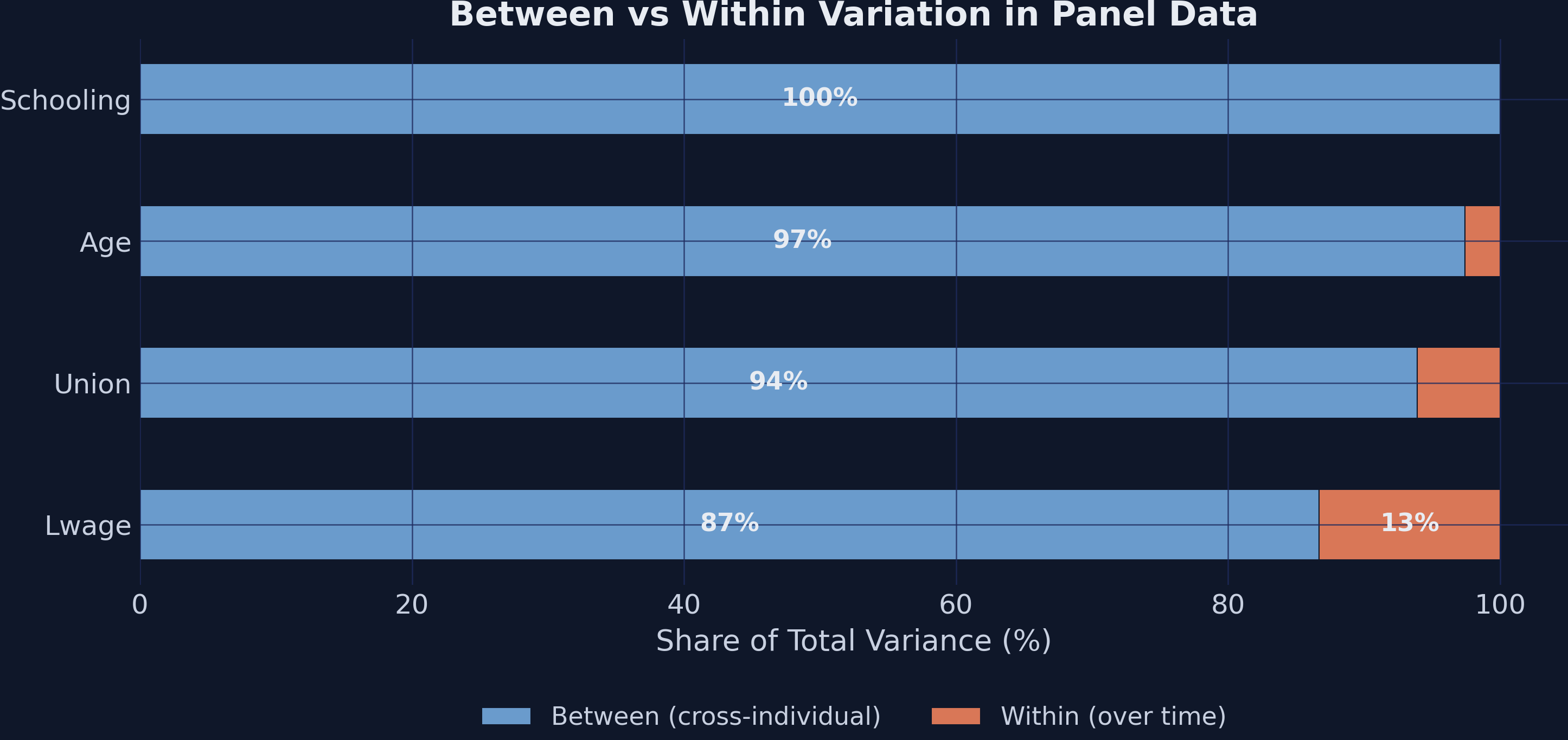
94% of union variation is between workers — only 9.1% is within

Between vs within variance shares for the four key variables. Union is 93.9% between; schooling is 100% between (zero within).

Fixed effects only use the within part. For union that is a thin 9.1% slice of total variance. Schooling has zero within-variation (nobody’s education changes across two years), so FE mechanically drops it. The consequence: FE standard errors will be much larger than POLS — the FE-vs-RE choice is about precision as much as bias.

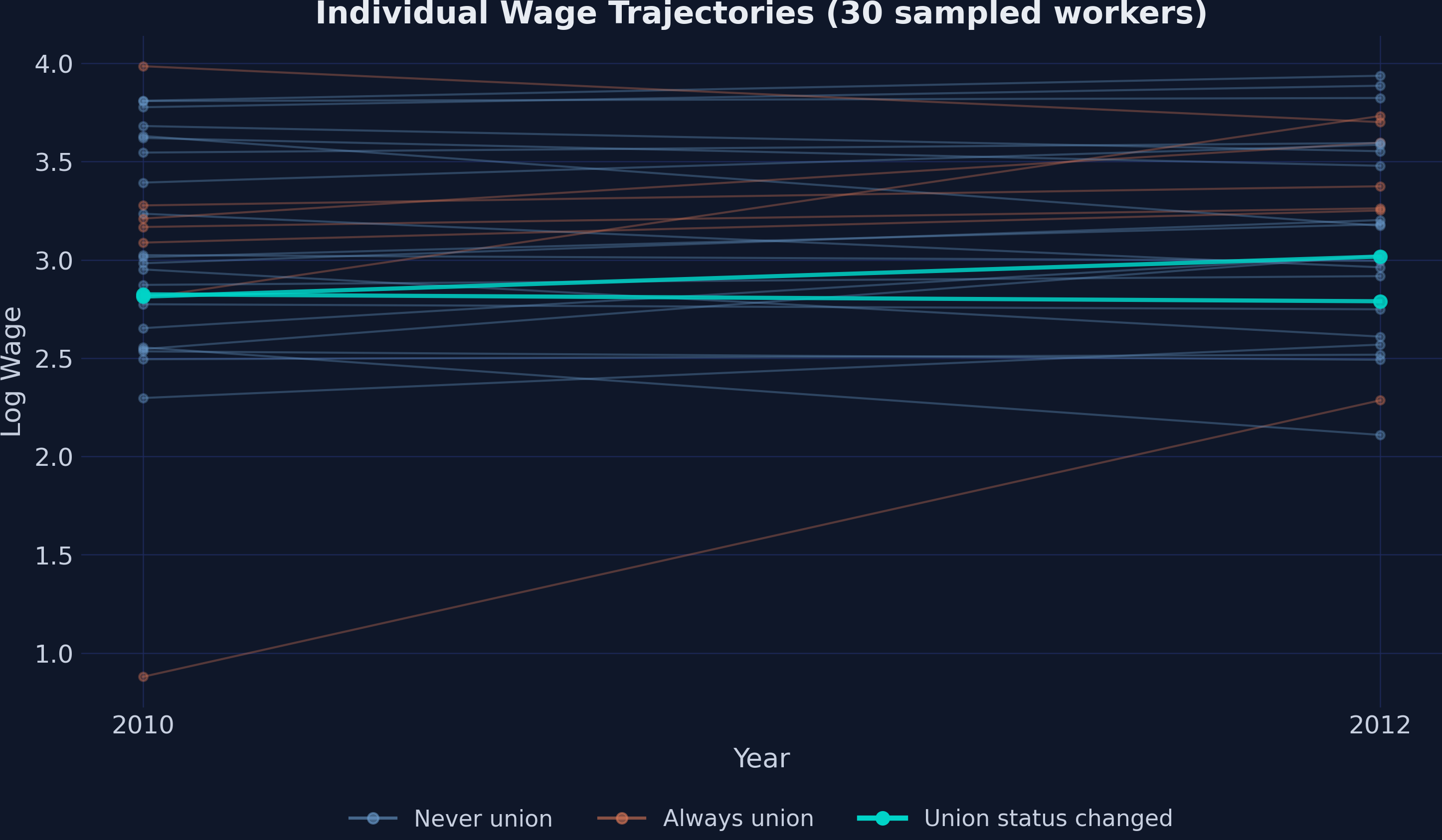
Only the workers who switch status identify the within estimators

Log-wage trajectories for 30 sampled workers. Teal lines change union status; orange/blue lines never do.

Most lines are flat-colored — always-union (orange) or never-union (blue). Only the teal “changer” lines carry identifying information for FE, FD, and Mundlak. Read only the teal lines and you have run fixed effects; ignore them and you have run a between estimator. The cross-sectional-vs-within tension is literally a question of which lines you choose to read.

Pooled OLS — the naive baseline — reports a 7.5% premium

fit_pols = pf.feols("lwage ~ union", data=df, vcov="HC1")
print(fit_pols.coef()["union"])   # 0.0750
# Union coefficient: 0.0750  (SE 0.0231)

Highly significant (\(t \approx 3.25\)) — and almost certainly biased if ability selects out of union jobs.

POLS treats every worker-year as independent, ignoring the panel. 7.5 log points, SE 2.3. This is the textbook cross-sectional answer and the number a naive analyst reports. The rest of the post is a tour through ways of subtracting the selection bias out. Between is its near-twin (0.066) because 94% of union variance is between-worker.

First-differencing erases \(\alpha_i\) and triples the estimate to 0.211

\[y_{i,2012} - y_{i,2010} = \beta\,(x_{i,2012} - x_{i,2010}) + (u_{i,2012} - u_{i,2010})\]

The worker-specific effect \(\alpha_i\) — ability, schooling, gender — cancels in the subtraction. What is left is identified only by workers who changed union status.

FDFE \(= 0.2113\) (SE 0.079); the SE is \(3.4\times\) larger than POLS — the switcher-only signature.

Start from y_it = α_i + β x_it + u_it; difference across the two periods and α_i drops out. The point estimate is almost three times POLS (0.211 vs 0.075) with a wide CI [≈0.06, 0.37] that still excludes zero. Workers who switch into unions are a different population from always-union workers, so the within parameter is genuinely different — and arguably cleaner.

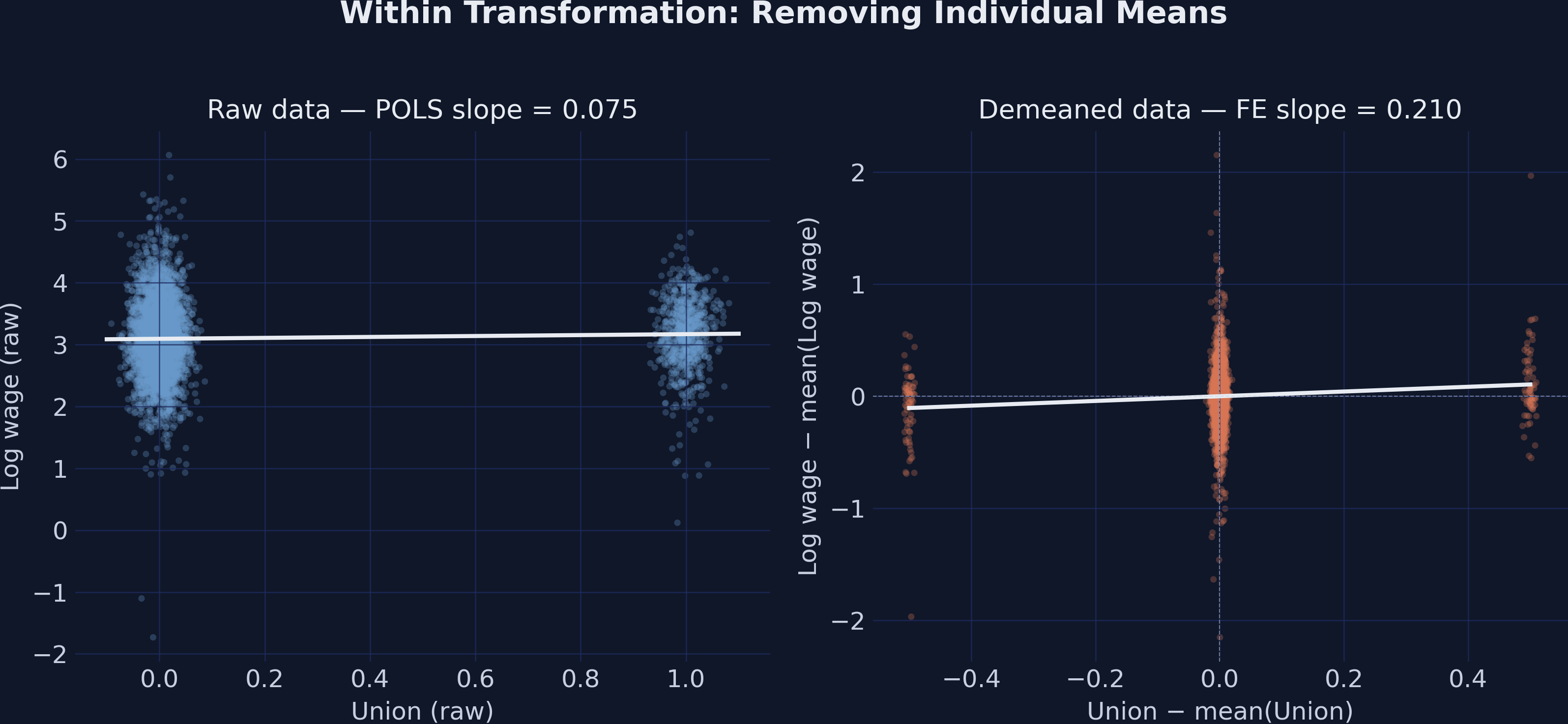
The within transformation demeans the data — and the slope steepens to 0.21

Within transformation: raw scatter with the shallow POLS slope (left); demeaned scatter with the steeper FE slope through the origin (right).

Same observations, two pictures. Left (raw): POLS slope ≈ 0.08, dragged down because union and non-union mean wages sit close together. Right (demeaned): FE slope ≈ 0.21, identified only by the points that move off the origin — the switchers. The within estimator subtracts each worker’s mean, so α_i vanishes; OLS on the demeaned data gives the FE coefficient.

Three recipes, one number: FD, demeaning, and dummy FE all give 0.2103

fit_fe   = pf.feols("lwage ~ union | ID", data=df, vcov="HC1")        # absorbed FE
fit_dvfe = pf.feols("lwage ~ union + C(ID_str)", data=df, vcov="HC1") # 2,198 dummies
# Both → 0.2103;  FDFE → 0.2113 (the +0.001 is an intercept-driven year trend)

Within transformation, first-differences, and dummy-variable FE are three recipes for the same dish. Absorption (| ID) is just the fast one.

DVFE with N−1 = 2,198 worker dummies recovers 0.2103 exactly. Modern software prefers absorption purely for speed: 2,199 dummies still runs fast, but at N = 100,000 the dummy spec is prohibitive while absorbed FE stays trivial. The FDFE +0.001 gap closes once we add a year effect — that is two-way FE, next.

Two-way FE absorbs year shocks and lands at 0.2129 — closing the FD–FE gap

fit_twfe = pf.feols("lwage ~ union + age | ID + year", data=df, vcov={"CRV1": "ID"})
# Union coefficient: 0.2129  (SE 0.0793)

Absorbing the year effect removes the aggregate wage trend FD’s intercept was capturing. Time-invariant regressors (schooling, female) are silently absorbed.

TWFE = 0.2129, all but identical to one-way FE because with T = 2 the time effect is small. The +0.002 vs FE is exactly the trend FD’s intercept absorbed. You cannot identify the effect of something that does not change within a worker — which is why applied researchers reach for CRE/Mundlak when they want within identification AND coefficients on time-invariant variables.

Random effects bets on no-correlation — and is pulled toward POLS at 0.109

exog = sm.add_constant(df_re[["union"]])
fit_re = RandomEffects(df_re["lwage"], exog).fit(cov_type="robust")
# Union coefficient: 0.1092  (SE 0.0299)

RE is a variance-weighted average of between and within. With only 9% within, it leans toward the between picture — and SE is \(2.7\times\) tighter than FE.

RE treats α_i as a random draw uncorrelated with the regressors and uses GLS to blend within and between efficiently. Here it lands at 0.109, squarely between POLS (0.075) and FE (0.210), leaning toward POLS because within variation is thin. The SE (0.030) is striking — but that precision is real only if individual effects are uncorrelated with union status. The FE–POLS gap suggests they are not, so the precision is bought with bias.

The Hausman test fails to reject RE — but only because FE is noisy

\[H = (\hat\beta_{\mathrm{FE}} - \hat\beta_{\mathrm{RE}})'\,[V_{\mathrm{FE}} - V_{\mathrm{RE}}]^{-1}\,(\hat\beta_{\mathrm{FE}} - \hat\beta_{\mathrm{RE}}) \sim \chi^2(k)\]

If FE and RE disagree a lot, \(H\) is large and RE is suspect. Here \(H = 1.79\), \(p = 0.180\) — fail to reject.

But \(H\) has low power exactly when within variation is thin: a noisy FE inflates \(V_{\mathrm{FE}}\) and shrinks \(H\) mechanically.

β_FE − β_RE = +0.101, a real gap, yet H = 1.79 on 1 df gives p = 0.180 > 0.05, so the textbook script says “use RE.” Take that verdict with a grain of salt: the large V_FE in the denominator is doing the work, not RE’s consistency. The Mundlak alternative tells the same story with more nuance, next.

Mundlak recovers the FE coefficient and flags negative selection

\[y_{it} = \alpha + \beta\,x_{it} + \gamma\,\bar{x}_i + u_{it}\]

Add each worker’s mean union exposure \(\bar{x}_i\), then run RE. The within coefficient \(\beta\) equals FE; the mean coefficient \(\gamma\) tests whether \(\alpha_i\) correlates with \(x\).

CRE within \(= 0.2103\) (matches FE exactly); Mundlak term \(\gamma = -0.144\), \(p = 0.072\) — borderline, hinting at negative selection.

Mundlak (1978) proved β here is numerically identical to FE — and it is, to four decimals (0.2103). The γ on union_bar is −0.144, p = 0.072: workers with higher average union exposure earn less even after conditioning on within changes, consistent with lower-wage workers selecting into unions. Same direction as Hausman, but it reaches the borderline zone because it doesn’t fight the same noise penalty.

The Resolution

Act III

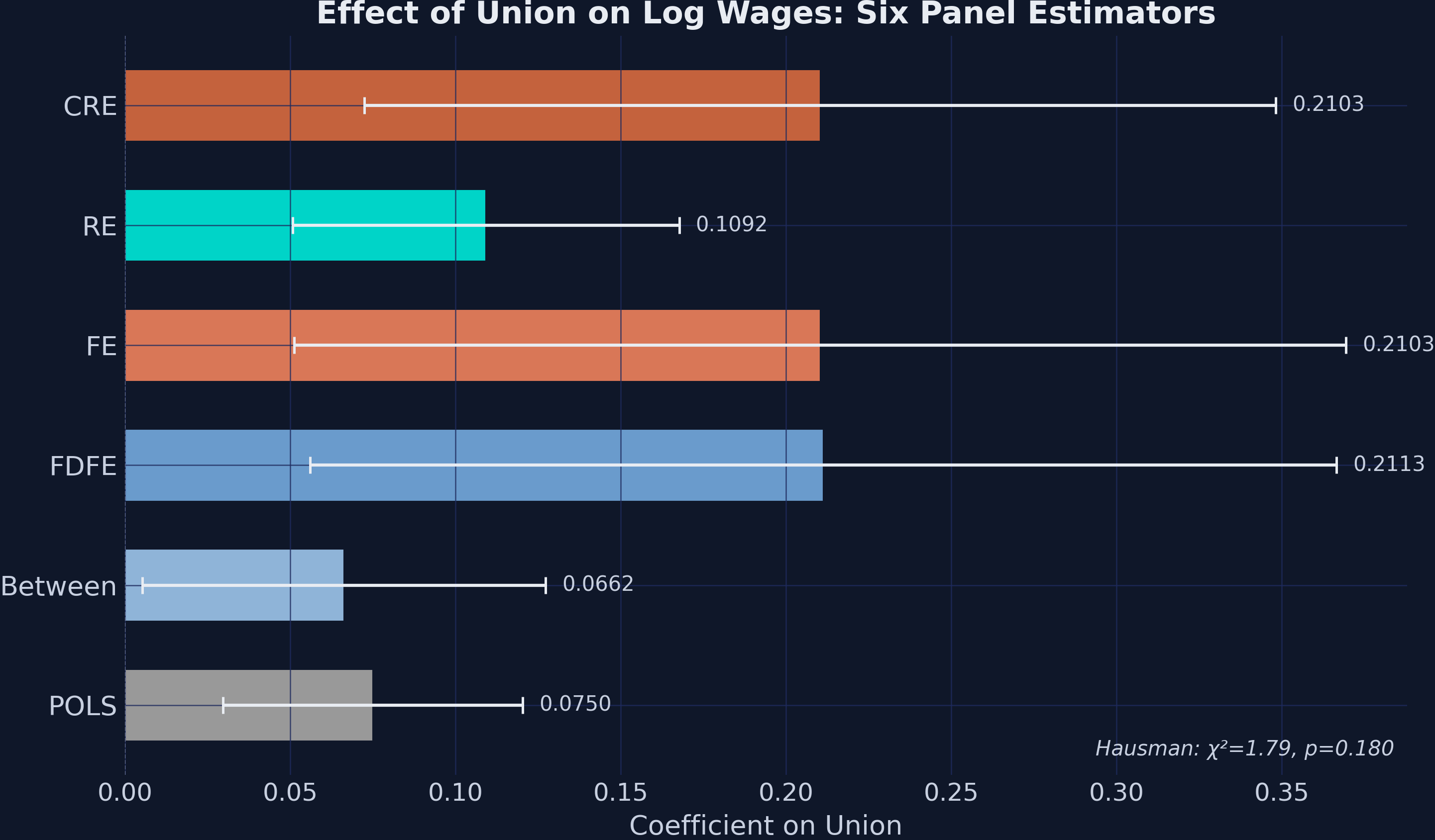
Within-worker, joining a union pays 0.21 log points — nearly triple the naive 0.075

0.210

\(\hat\beta_{\mathrm{FE}}\) on union (SE 0.081) — vs pooled OLS 0.075; FDFE, TWFE, and CRE all agree near 0.21

The Act-III payoff. Cross-sectional methods say 7–11%; within methods say ~21%. The factor-of-three gap is the empirical signature of selection on unobservables: higher-ability workers are less likely to be unionized in this sample, so cross-sectional comparisons understate the within-worker payoff to joining a union.

Two camps, three-fold apart — and the gap is selection, not noise

Method	Coef	SE	Variation used
POLS	0.0750	0.0231	all (ignores panel)
Between	0.0662	0.0311	cross-sectional means
RE	0.1092	0.0299	GLS between + within
FDFE	0.2113	0.0792	within differences
FE	0.2103	0.0812	within demeaned
CRE	0.2103	0.0703	RE + Mundlak (= within)

Cross-sectional 7–11% · within ~21%. Standard errors swing inversely — the within camp is noisier but causally cleaner.

The payoff table. The six methods cluster into two camps roughly three-fold apart. Cross-sectional methods are 2–3× more precise but identify a biased (under our hypothesis) parameter; within methods are noisier but cleaner under weaker assumptions. Reporting both estimands side by side is more honest than picking one.

Adding controls leaves the four-camp gap intact

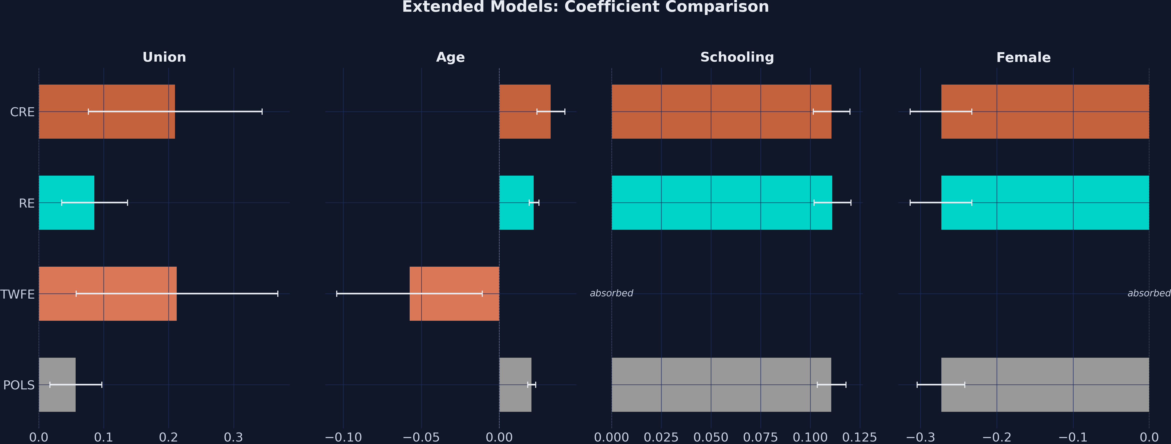
Extended models — union, age, schooling, female across POLS / TWFE / RE / CRE. The within premium survives controls.

With age, schooling, female, and year dummies, POLS drops to 0.057 (controls absorb some confounding), but TWFE and CRE still report ~0.21. Schooling (+11.1%/yr) and the female penalty (−27.3 log pts) are stable across POLS/RE/CRE because they are time-invariant — and absorbed by FE. The TWFE age coefficient flips to −0.058, a T = 2 artifact (age is collinear with the year dummy), not a real age–wage relationship.

Does FE make this causal? No — strict exogeneity still carries the weight

Objection. Within estimators just net out fixed traits — they can’t manufacture identification.

Response. Correct. FE/FDFE/TWFE/CRE target the ATE for union switchers only — and only under strict exogeneity given the worker fixed effect.

Steelman, don’t strawman. They remove time-invariant confounders, not time-varying ones — a promotion that coincides with joining a union still biases the within estimate. POLS and Between carry no causal reading absent unconfoundedness. Fixed effects discipline the comparison; they do not relax identification. The within estimand is local — it is identified off the ~9% of workers who switched status — and rests on strict exogeneity conditional on α_i. Reporting both the within and cross-sectional estimands, as the post does, is the honest move.

In low-power settings, lead with CRE/Mundlak — it dominates Hausman

p = 0.072

Mundlak term — borderline, more honest than Hausman’s confident p = 0.180 “fail to reject”

CRE/Mundlak gives you three things in one regression: the FE coefficient on the time-varying treatment, the RE framework that retains schooling and gender, and a built-in specification test (the t-stat on the Mundlak term) that beats Hausman when within variation is thin. The cost — one extra regressor per time-varying covariate — is essentially free in modern software.

Let the within variation, not the pooled average, tell you what a treatment does.

The single takeaway. When selection on unobservables is plausible, the gap between 0.075 and 0.210 is the whole story — and CRE/Mundlak is the specification that recovers the within answer while keeping the RE machinery and an honest specification test.