Carbon Taxes and CO2 Emissions

A synthetic-control analysis of Sweden’s 1991 reform, in Python

−11.3%synthetic Sweden, CO2 per yr

3×tax vs price response

6donor countries

Carlos Mendez

Nagoya University (GSID)

June 11, 2026

The Tension

Act I

Sweden’s emissions rose 0.55 t/capita after the carbon tax — or did they?

In 1991 Sweden put one of the world’s first prices on carbon. A naive before/after says emissions went up 0.55 t per capita.

The economy also grew, the fleet changed, oil prices swung. Compared to what would have happened anyway?

The central problem of causal inference in one slide. Sweden’s raw post-1990 mean is higher than its pre-1990 mean only because the post window runs to 2005 and the whole economy grew. The naive number is an arithmetic fact and a useless causal answer. We need a counterfactual Sweden — one that never got the tax. That is the entire job of the rest of the deck.

The spoiler: Sweden flattens after 1990 while its synthetic twin keeps climbing

Sweden (actual) vs Synthetic Sweden, a weighted blend of donor countries. Lines overlap before 1990; they split after.

Don’t explain the construction yet — just plant the picture. Before 1990 the two lines are on top of each other; that is the fit we earn. After 1990 the gap is the effect we will defend with three placebo tests. We come back to this image as the payoff in Act III.

Where we’re going

• Three estimators, escalating discipline: naive → DiD → synthetic control
• Building Synthetic Sweden from a donor pool, then reading the gap
• Three placebo tests: in-time, in-space, leave-one-out
• Was it just a recession? A second synthetic control on GDP
• Why consumers responded: tax vs price elasticities (OLS / IV)

The Investigation

Act II

The lab: 15 OECD economies, 46 years, 30 of them before the reform

• Outcome — per-capita transport CO2 in metric tons, 1960–2005
• Treated unit — Sweden; the carbon tax switches on in 1991
• Donor pool — 14 other advanced economies, untreated
• Window — 30 pre-treatment years to fit, 16 post-treatment to measure

The long pre-period is a structural advantage. It lets us check the counterfactual before the policy — where the gap should be zero.

The estimand is the ATT: how much lower were Swedish emissions than a no-reform Sweden?

\[\tau_t = Y^{\text{obs}}_{\text{Sweden},t} - \hat Y^{N}_{\text{Sweden},t}, \qquad \hat Y^{N}_{\text{Sweden},t}=\sum_{j=2}^{J+1} w_j\, Y_{jt}\]

We never observe \(\hat Y^{N}\) — Sweden without the tax. Synthetic control estimates it as a weighted blend of donors.

\(Y^{\text{obs}}\) is what happened; \(\hat Y^{N}\) is the counterfactual; the gap \(\tau_t\) is the treatment effect on the treated.

ATT, not ATE: we estimate the effect for the one treated unit, Sweden, not an average over a population. The donor weights w_j are non-negative and sum to one, so the synthetic is a genuine convex combination — an interpolation among real countries, never an extrapolation. That convexity is what makes the method credible.

DiD against Denmark flips the naive sign — but parallel trends fail in the pre-period

Comparison	\(\hat\tau\) (ATT)	SE	\(p\)
Naive Sweden pre/post	+0.55	0.08	0.00
DiD vs Denmark	−0.140	0.116	0.23
DiD vs OECD pool (cluster SE)	−0.214	0.083	0.02

Differencing against a control flips +0.55 to negative — but one control is underpowered, and the pre-trends don’t line up.

Denmark alone reproduces Andersson’s −0.140 exactly, but p = 0.23: one control is a noisy counterfactual. The full 14-country pool with cluster-robust SEs tightens to −0.214, p = 0.02. The catch: the pre-1990 CO2 plots show Sweden and the OECD mean were not on parallel trends. DiD’s key assumption is visibly violated — which is exactly why we move to synthetic control, which does not need parallel trends, only a good pre-period fit.

Synthetic control chooses the donor weights by data, under two hard constraints

\[w^* = \arg\min_{w}\ (X_1 - X_0 w)^\top V (X_1 - X_0 w) \quad \text{s.t.} \quad w_j \geq 0,\ \sum_j w_j = 1\]

\(X_1\) are Sweden’s pre-treatment predictors; \(X_0\) the donors’. The optimiser also picks \(V\) to minimise pre-period CO2 prediction error.

Non-negative weights that sum to one \(\Rightarrow\) the synthetic is a convex blend — no extrapolation, no parallel-trends assumption.

Two nested optimisations: pick the donor weights w given the predictor-importance matrix V, then pick V so the resulting synthetic best tracks Sweden’s actual CO2 in the pre-period. The constraints are the whole point — they force the counterfactual to live inside the convex hull of real countries.

pysyncon picks the same six donors as Andersson’s R code

controls = [c for c in countries if c != "Sweden"]
dataprep = Dataprep(
    foo=panel, dependent="CO2_transport_capita",
    predictors=["GDP_per_capita", "vehicles_capita",
                "gas_cons_capita", "urban_pop"],
    treatment_identifier="Sweden", controls_identifier=controls,
    time_optimize_ssr=range(1960, 1990),
)
synth = Synth()
synth.fit(dataprep=dataprep, optim_method="Nelder-Mead")
print(synth.weights().sort_values(ascending=False).head(6))
# Denmark .29 · Belgium .27 · New Zealand .15 · Greece .11 · US .10 · Switzerland .08

Two objects do all the work: Dataprep packs the panel into the matrices the optimiser needs; Synth.fit runs the nested optimisation. The donor set is identical to Andersson’s R run; the percentage shares differ a little because scipy’s Nelder-Mead and R’s kernlab interior-point solver are different optimisers reaching the same family of solutions.

Six donors carry 100% of the weight — Denmark and Belgium dominate

Donor weights for Synthetic Sweden. Six countries share all the weight; the other nine get essentially zero.

Denmark 29% and Belgium 27% together are over half — small, advanced European economies with Sweden-like income, urbanisation, and energy mix. New Zealand brings the urbanisation match; Greece, the US, and Switzerland fill in. Concentrated weights like these signal a tight fit. Weights spread thinly across many donors would be a red flag that no good counterfactual exists in the pool.

Pre-1990 the gap is near zero; post-1990 it widens monotonically to −0.36 t

Year-by-year gap, Sweden minus Synthetic Sweden. Flat before the reform; a widening wedge after.

The pre-period gap hugging zero is the validation: the synthetic mimics both the level and the trend of real Swedish emissions before any policy. After 1990 the gap opens steadily — 2005 gap −0.36 t/capita (−15% vs the synthetic level), averaging −0.27 t/capita or −11.3% per year across the post window. About one ton of avoided per-capita CO2 every 3.7 years.

The headline: −11.3% per year for 16 years

−11.3%

average annual gap, Synthetic Sweden, 1990–2005 (2005 gap −0.36 t/capita, −15%)

This is the central estimate. It sits between the no-controls baseline and the noisy DiD numbers, and it matches Andersson’s reported range and the R tutor’s −10.9% within rounding. But the SCM optimiser is designed to make the treated unit look unique post-period — so a number alone is not enough. Placebo tests are the price of admission.

Falsification 1 — backdate the reform to 1980 and no fake gap appears

In-time placebo: fit as if the tax arrived in 1980. Sweden and its synthetic stay locked together.

We re-fit using only pre-1980 data and pretend the reform happened in 1980. If the SCM manufactured gaps from noise, one would show up here. It doesn’t — Sweden tracks its synthetic through 1990 with no divergence at the placebo date. The method does not invent gaps where no policy exists.

Falsification 2 — Sweden’s gap beats 14 of 15 placebo countries, p = 0.067

In-space placebos: re-run the SCM pretending each donor was treated. Sweden (bold) sits outside the grey bundle.

We re-run the whole SCM fifteen times, treating each country as if it were Sweden, and rank by the post-/pre-treatment MSPE ratio — dividing by pre-period fit so badly-fit units don’t get spurious credit. Sweden has the highest ratio of any unit. The permutation p-value is 0.067: only one in fifteen random reassignments is as extreme. With 15 donors, 1/15 ≈ 0.067 is the smallest p the design can deliver — and we hit it.

Falsification 3 — drop any single donor and the effect stays in 8.8%–13%

Leave-one-out: Synthetic Sweden recomputed dropping each high-weight donor in turn. All firmly negative.

Maybe one quirky donor — Denmark — drives everything? We re-fit six times, each excluding one high-weight donor. The reduction ranges from 8.8% (drop Switzerland) to 13% (drop Denmark); all six bracket the headline 11% and stay negative. Even the most conservative exclusion beats the unweighted DiD. The result is not a single-donor artefact. All three falsification tests pass.

Was it just a recession? Synthetic GDP overlaps actual GDP within $233 by 2005

Sweden’s actual GDP vs a separately-built Synthetic Sweden (GDP). The paths overlap throughout the post-period.

The standard objection: emissions fell because the early-1990s recession depressed driving, not because of the tax. Two answers. First, the CO2 gap never rebounds when GDP recovers after 1993 — a recession story predicts a rebound. Second, a separate synthetic control with GDP as the outcome (Denmark 61%, Norway 20%, Finland 10%, US 9%) tracks Sweden’s actual GDP to within $233 per capita by 2005, under 1% of the level. No measurable growth penalty. The policy worked and the economy was fine.

Pass-through is complete: consumers paid 1.15 of every tax krona at the pump

\[\Delta p^*_t = \beta_0 + \beta_1\, \Delta \Theta_t + \beta_2\, \Delta T_t + \varepsilon_t, \qquad \hat\beta_2 = 1.15\ (\text{SE } 0.15)\]

The 95% CI is roughly \([0.85, 1.45]\) — it contains 1. We cannot reject full pass-through.

If oil firms had absorbed the tax, the price signal never reaches drivers. They didn’t — so the behavioural channel is real.

Regressing the year-on-year change in the retail price on changes in the oil price and the energy-plus-carbon tax. β₂ = 1.15, statistically indistinguishable from one. Working in first differences strips out time-invariant levels and isolates the response to new tax movements. This matters: the demand elasticities below are responses to a real pump-price change, not to a hidden refiner absorption.

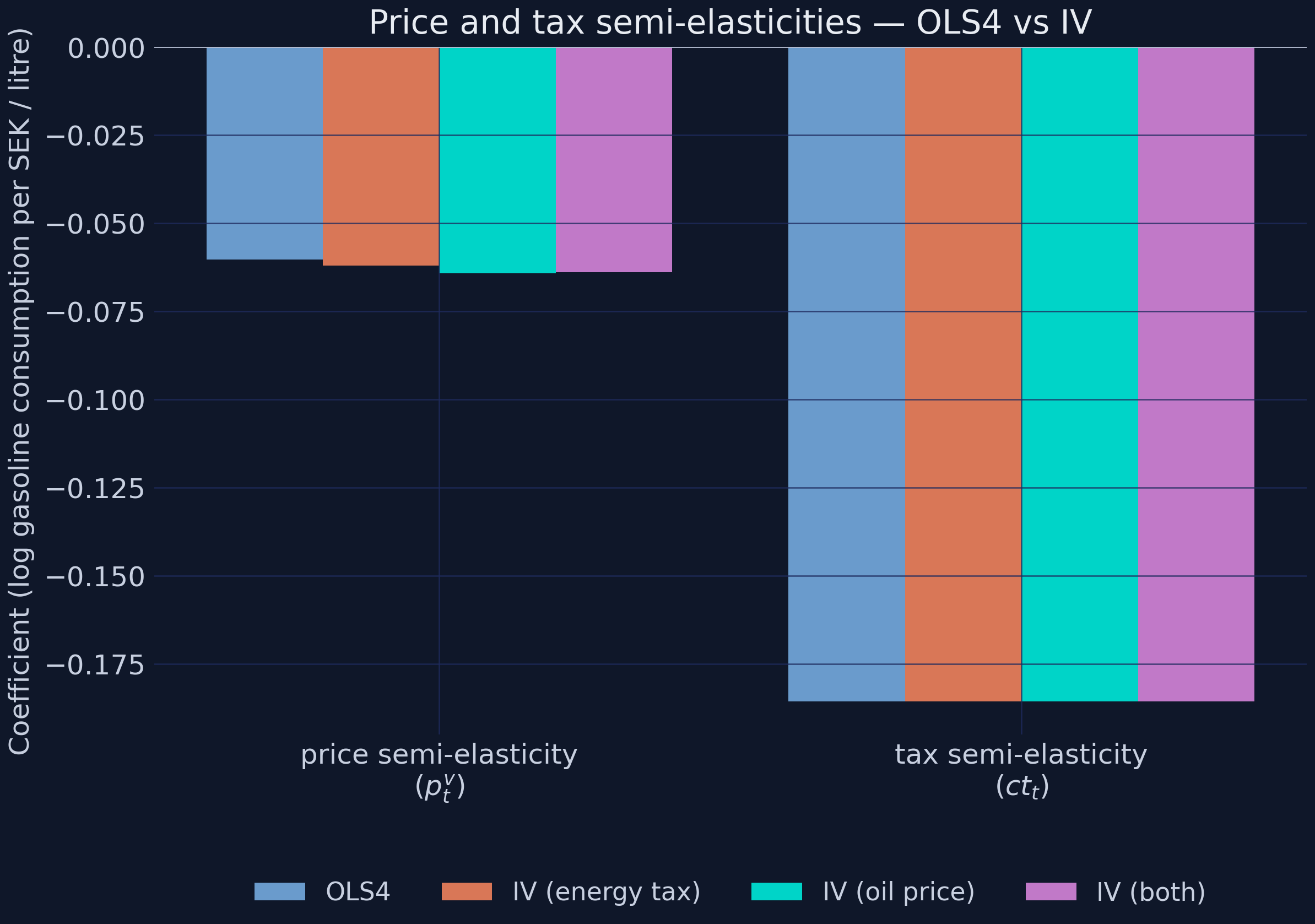
Consumers respond ~3× more strongly to a tax krona than to a price krona

Price semi-elasticity

• \(\hat\beta_{\text{price}} = -0.060\)
• +1 SEK/litre real price \(\Rightarrow\) −6% gasoline use
• stable across OLS1–OLS4
• IV (oil price): −0.064

Tax semi-elasticity

• \(\hat\beta_{\text{tax}} = -0.186\)
• +1 SEK/litre real tax \(\Rightarrow\) −18.6% gasoline use
• stable across OLS1–OLS4
• IV: pinned at −0.186

Salience + permanence: a tax is announced, debated, and persistent; a price drift is just a number on a billboard.

Log-level model, so coefficients are semi-elasticities. The 3-to-1 ratio is the section’s headline behavioural finding, and it barely moves across four nested OLS specs or three IV variants. Newey-West HAC(16) SEs — matching Andersson’s Stata — are actually tighter than HC1 here. Both elasticities stay highly significant.

IV barely moves OLS — and that itself is informative

Price and tax semi-elasticities under OLS4 and three IV specifications. The tax coefficient is locked at −0.186.

We instrument the carbon-tax-exclusive price with the real oil price (Sweden is too small to move world oil) and the real energy tax (set on long policy lead times). The tax elasticity is −0.186 to four decimals across every spec; the price elasticity nudges from −0.060 to −0.064. Had OLS been badly endogenous, IV would have moved it. Andersson’s Wu-Hausman test cannot reject price exogeneity — so we read OLS4 as causal.

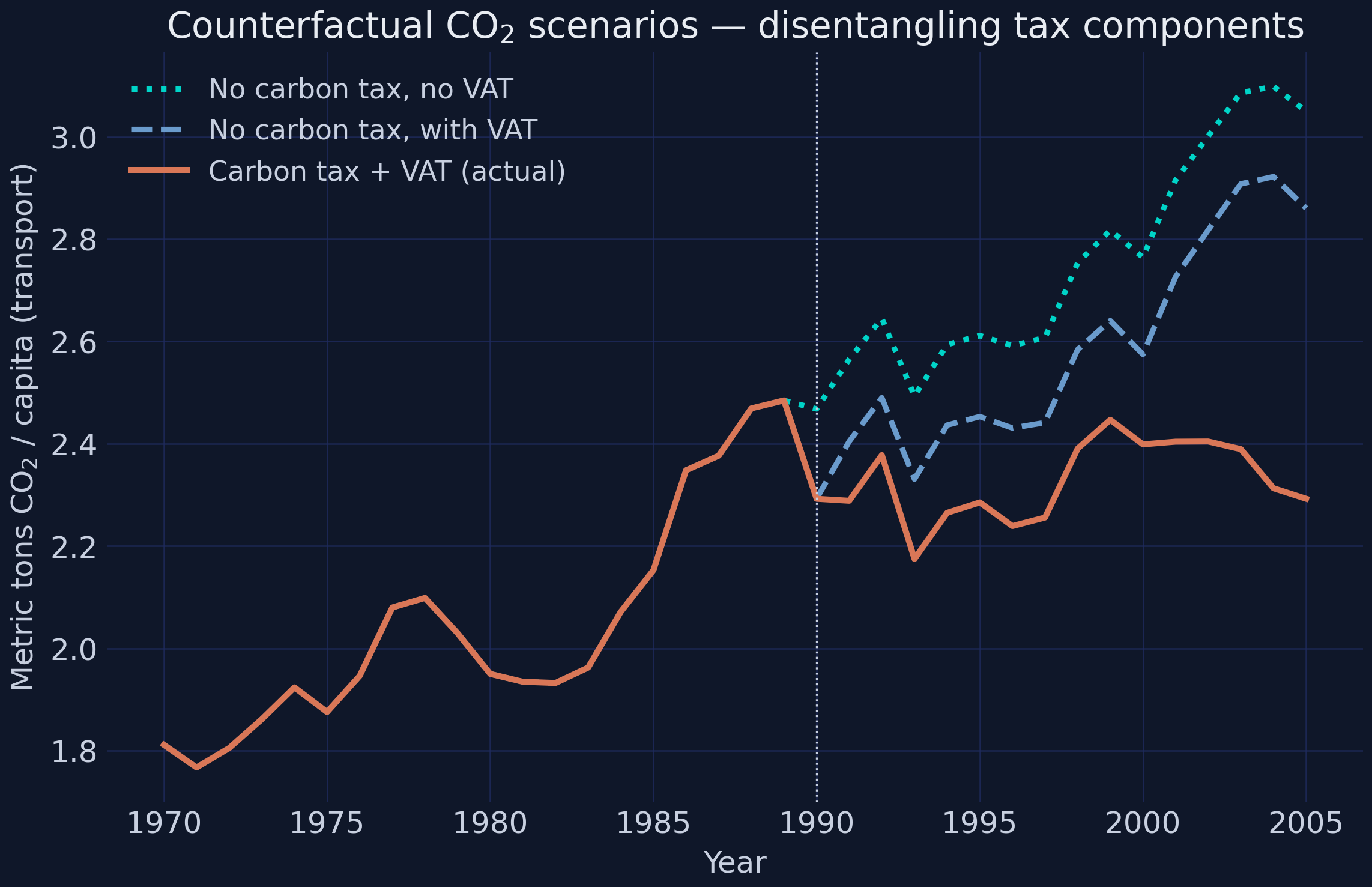
The carbon tax alone explains ~75% of the 2005 reform wedge

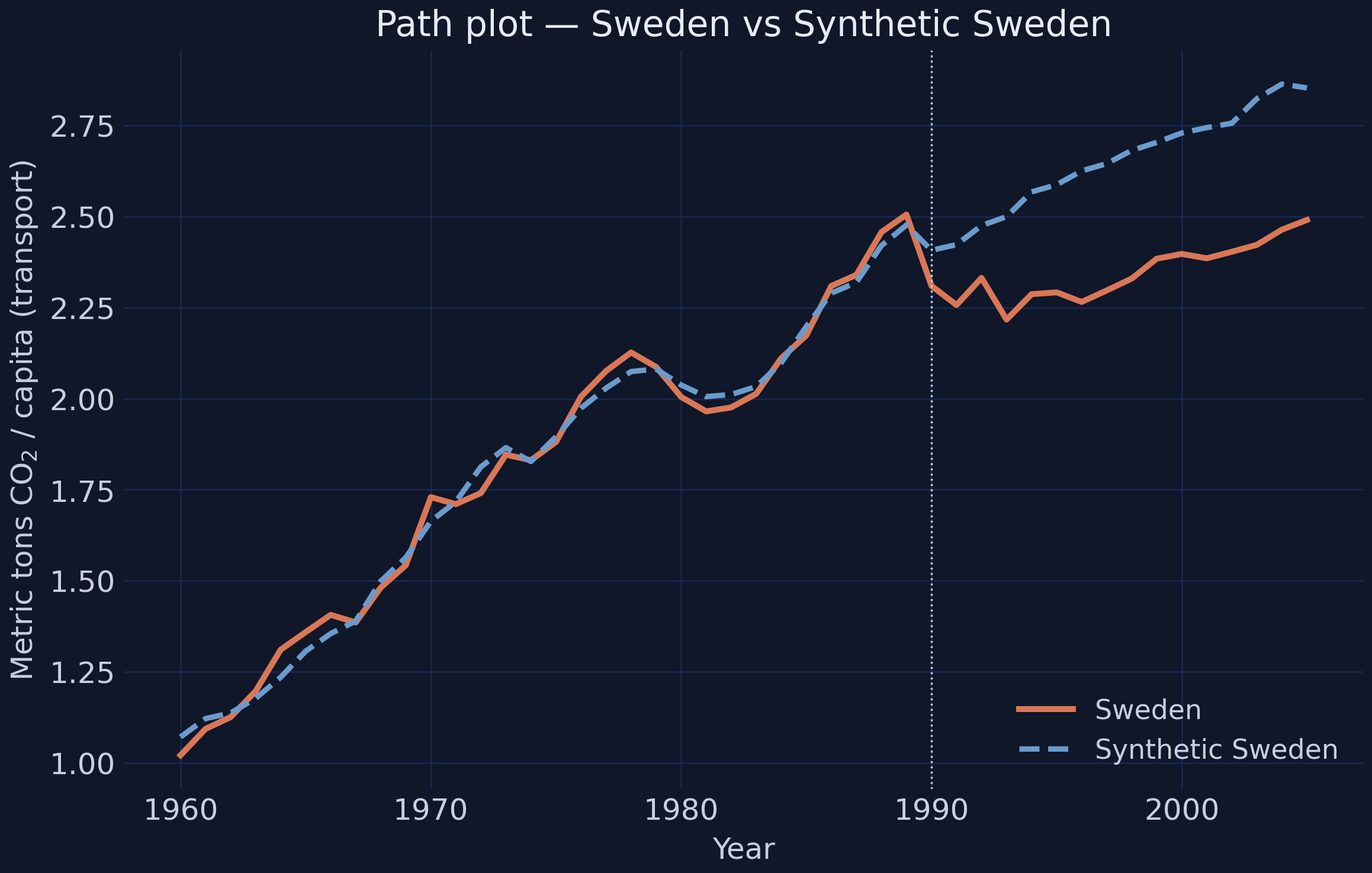
Three counterfactual CO2 paths. The orange-to-blue gap is the carbon-tax-only contribution; orange-to-teal adds the VAT.

The 1990/91 reform bundled a carbon tax, a new VAT on fuel, and a small energy-tax cut. Using Andersson’s pre-computed counterfactual paths, the carbon-tax-only wedge — between the actual line and the with-VAT-but-no-carbon-tax line — reaches −0.57 t/capita in 2005, about 75% of the total reform gap that year, and averages 9.5% of the no-carbon-tax-with-VAT baseline. The carbon tax does most of the work after 2000, when the rate is ratcheted sharply upward.

The Resolution

Act III

One sentence: the tax cut CO2 ~11% a year, at no measurable cost to growth

Quantity	Value	Reading
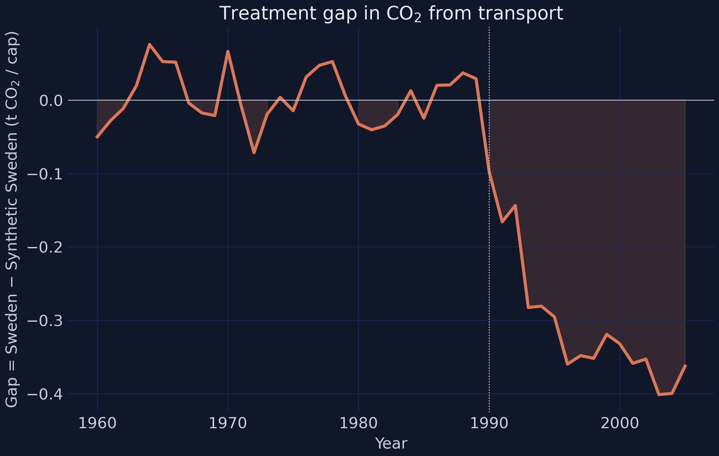
Synthetic gap, avg	−11.3%	CO2 cut ~a tenth, every year, 16 years
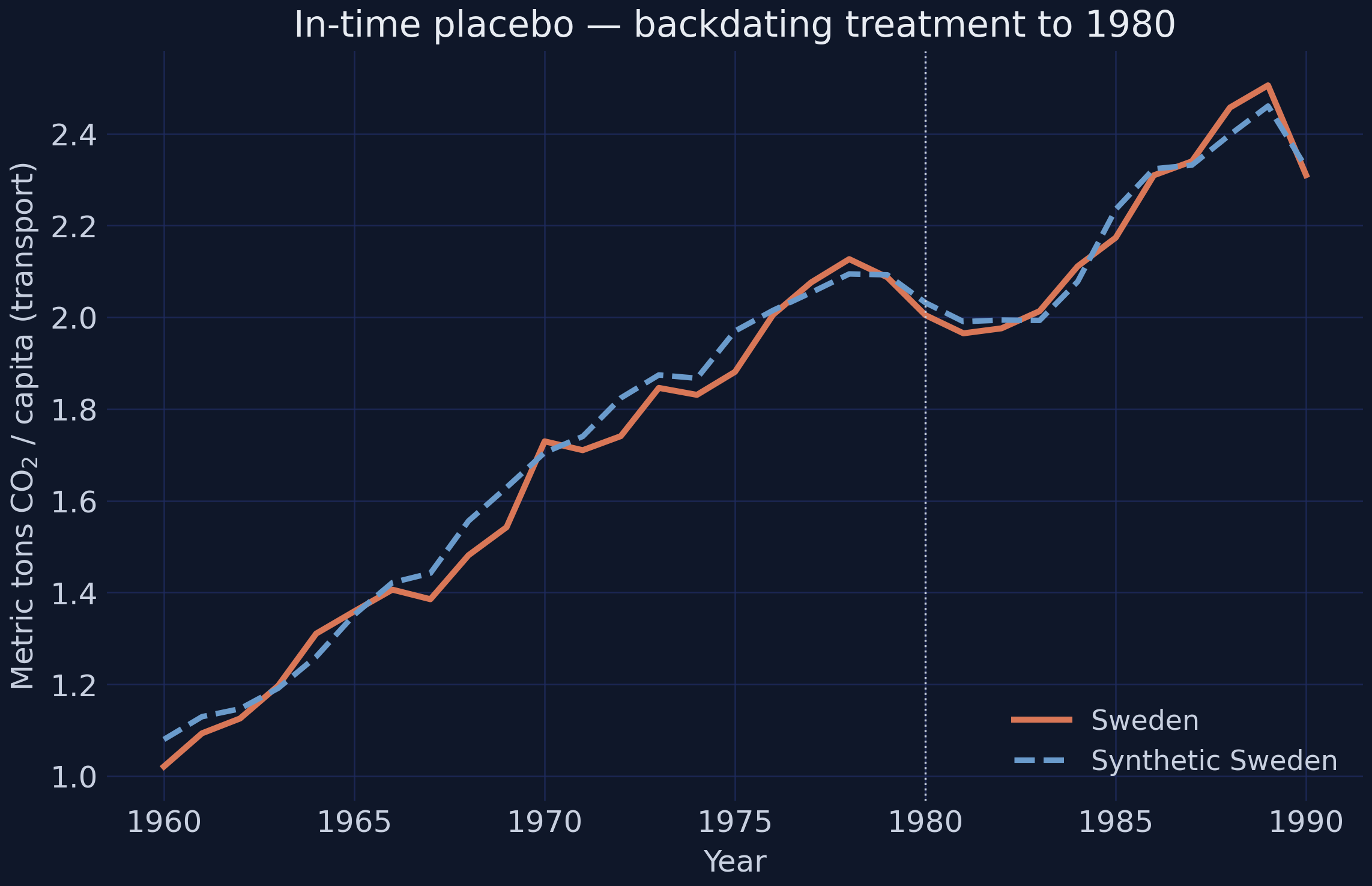
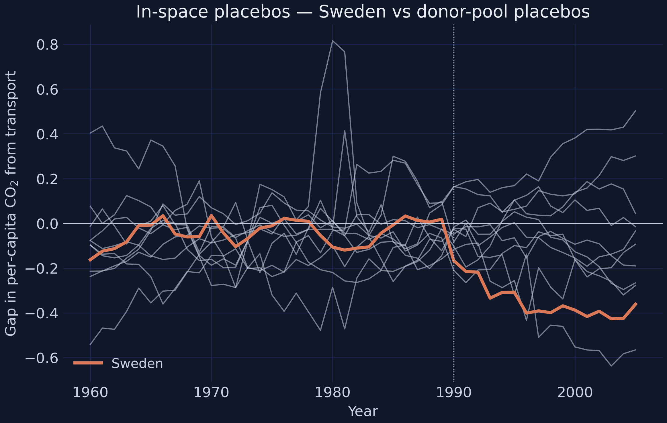
Permutation \(p\)	0.067	1 of 15 placebos is this extreme
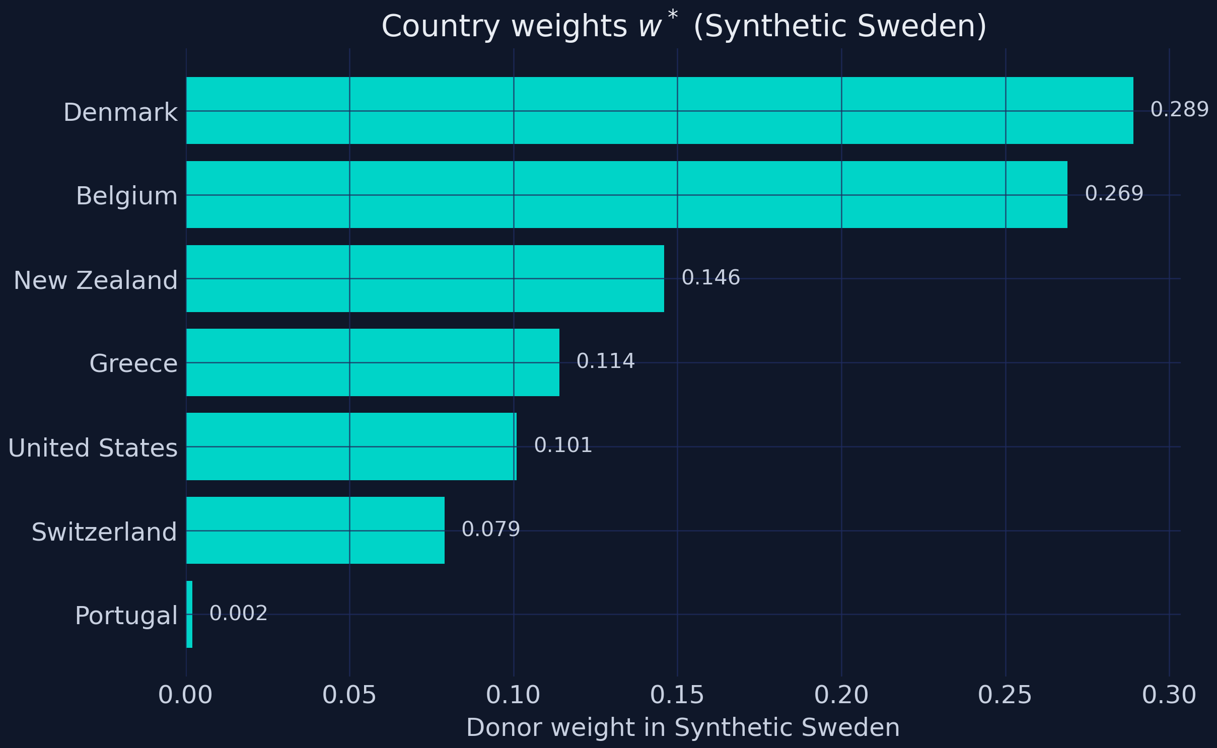
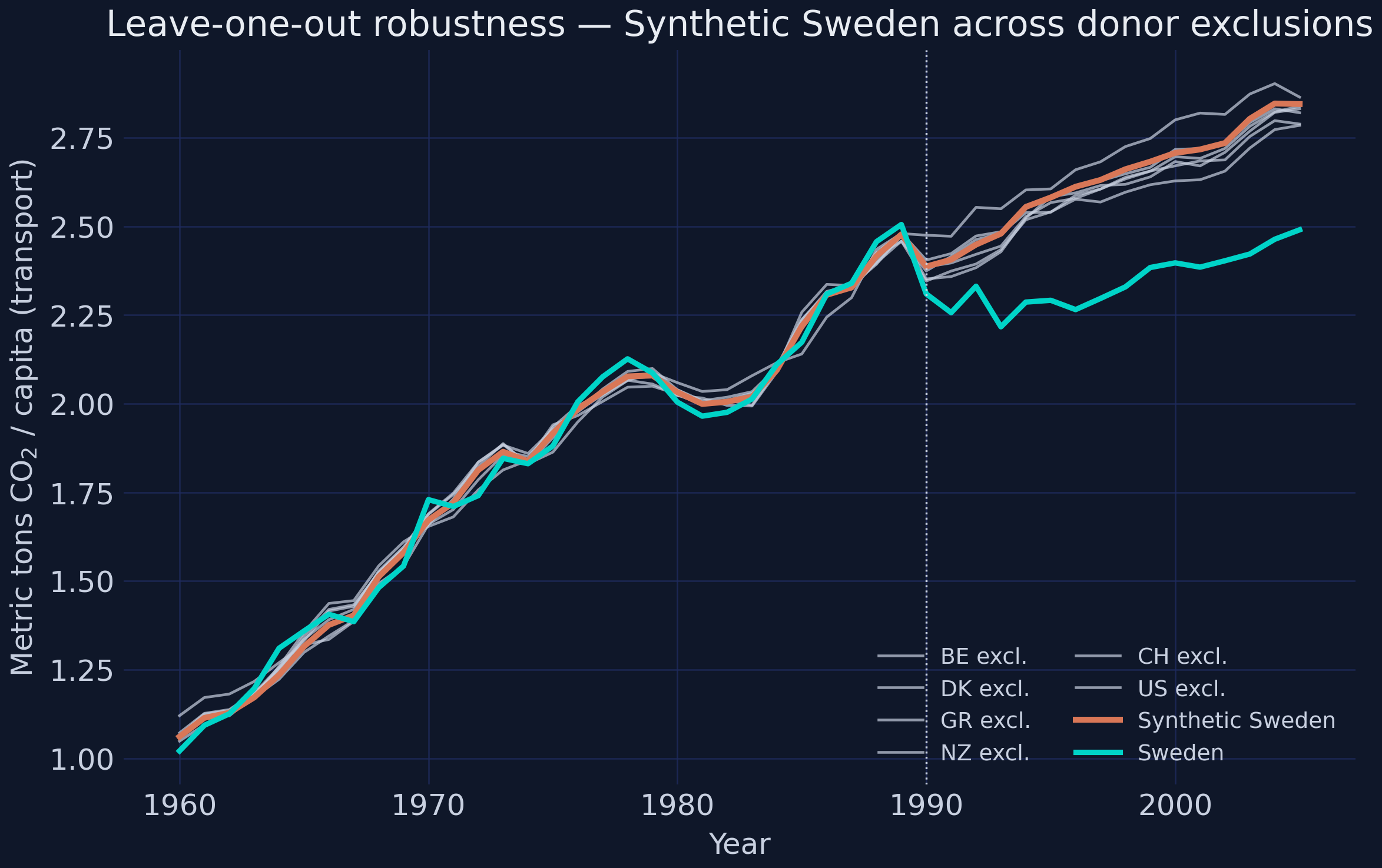
Leave-one-out	8.8%–13%	survives dropping any single donor
Tax vs price	3×	tax bites 3× harder per SEK
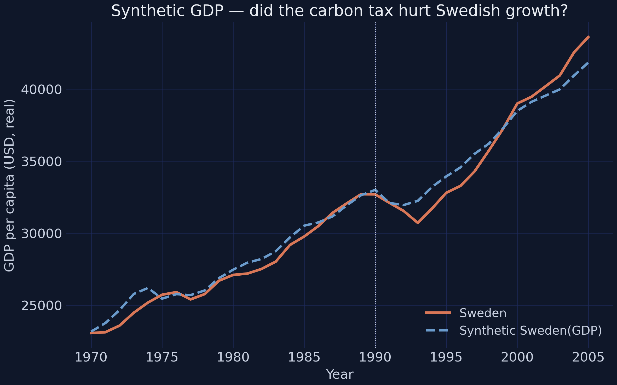
Synthetic GDP gap	< $233/cap	no detectable growth penalty

Five numbers, five independent pieces of evidence. The effect is large, robust to three falsification tests, not driven by any one donor, mechanistically explained by complete pass-through and a salient-tax response, and free of a growth penalty. This is what a credible synthetic-control case study looks like.

The strongest objection — and the answer

Objection. Sweden is one country, one observation. With 15 donors the smallest possible \(p\) is \(1/15 \approx 0.067\) — you hit the floor, not a clean rejection. And the analysis stops in 2005.

Response. All true, and stated plainly. But three independent falsifications point the same way, the GDP placebo rules out the recession story, and the demand-side mechanism is identified separately. The design under-claims by construction; the convergence of evidence is the argument, not any single \(p\).

Steelman, don’t strawman. Single-country external validity is genuinely limited; the donor pool caps the p-value; there’s no post-2005 EV-era data. None of this is hidden. The defence is that the SCM gap, three placebos, the GDP counterfactual, and the elasticity mechanism are independent and all agree — and the headline number is robust to every leave-one-out exclusion.

A salient, persistent, fully passed-through carbon tax cut emissions — without cutting growth.

The single takeaway, the resolution of the Act-I hook. The naive +0.55 was an illusion of confounding; the disciplined counterfactual reveals a −11.3% reduction that survives every falsification — and the economy was fine. Revenue-neutral tax swaps can deliver real emission cuts even when the average tax burden is unchanged, because the composition of taxes carries more behavioural weight than the level.