The Augmented Synthetic Control Method

Did the 2012 Kansas tax cut help? A single-unit ASCM tutorial

−0.040Ridge ASCM ATT · −3.9%

0.011estimated bias · a third of the effect

7donor states in synthetic Kansas

Carlos Mendez

Nagoya University (GSID)

June 11, 2026

The Tension

Act I

There is only one Kansas, and it took the treatment

In May 2012 Kansas enacted one of the largest state tax cuts in U.S. history — Gov. Brownback called it “a real-live experiment” in supply-side growth.

To judge it we need the Kansas that didn’t cut taxes. That Kansas does not exist. Where do we get the counterfactual?

This is the fundamental problem of causal inference with a single treated unit. We observe Kansas-with-the-tax-cut; we need Kansas-without-it. No state is a perfect twin, so we cannot just pick a comparison — we have to build one.

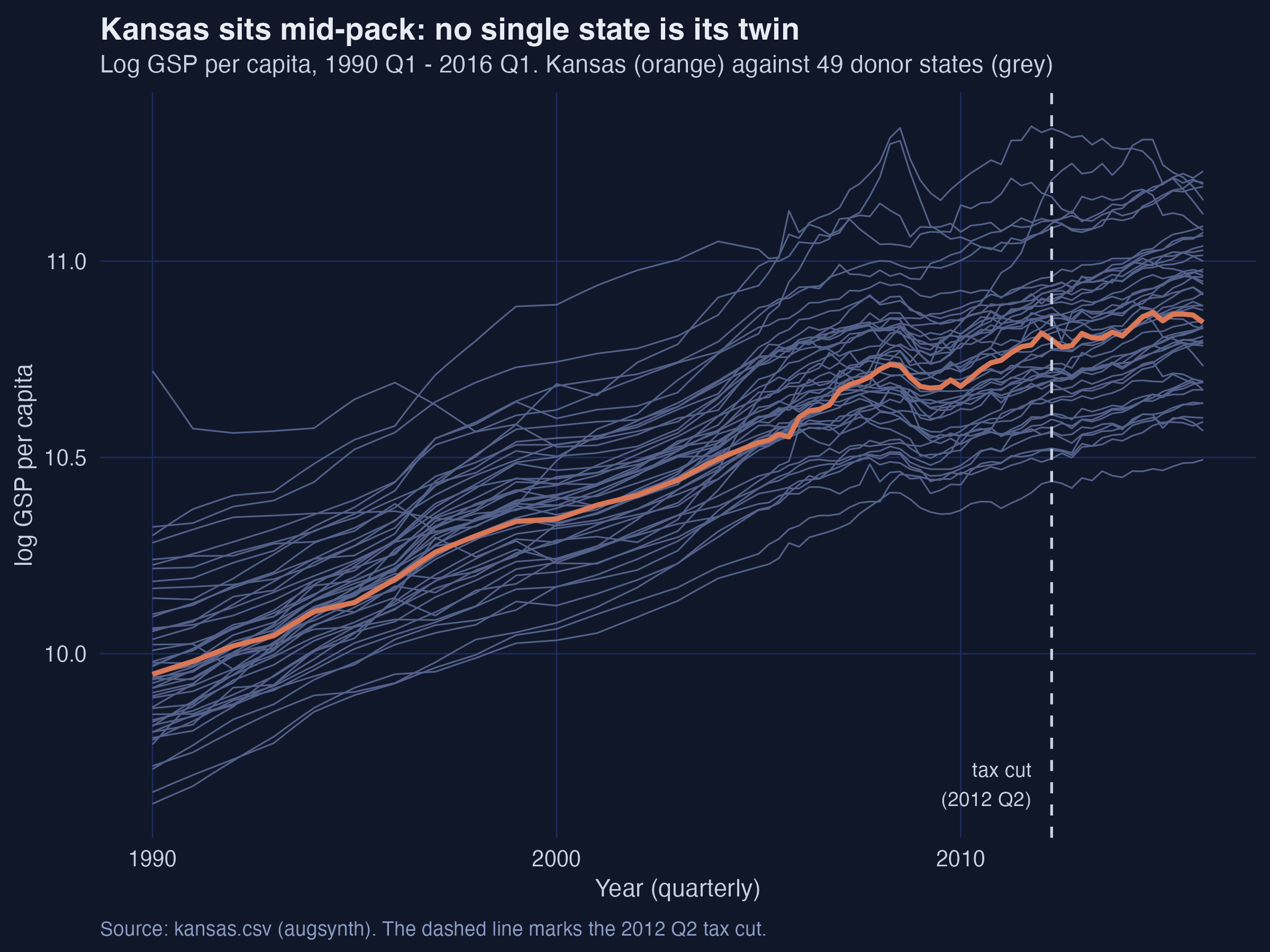
No single state is a Kansas twin — so we must build one

Log GDP per capita, Kansas (orange) vs the 49 donor states (grey), 1990–2016. The dashed line marks the 2012 Q2 tax cut.

Kansas sits squarely in the middle of the pack and rises with everyone for 26 years. No donor line lies on top of Kansas’s. The mid-2000s is where the lines fan apart and Kansas wanders — foreshadowing exactly where a convex blend will struggle.

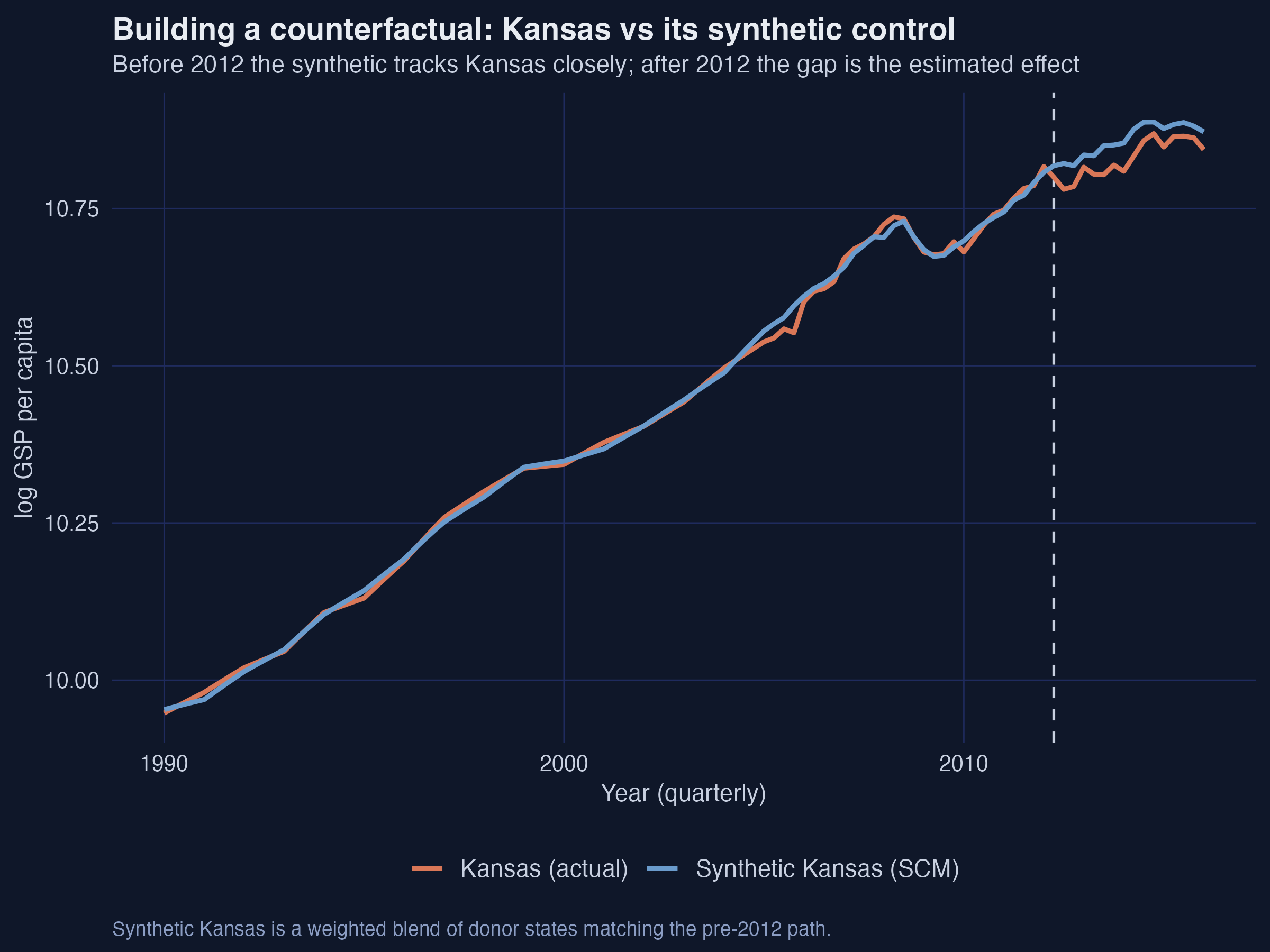
After 2012 Kansas slips below the synthetic control we build for it

Actual Kansas (orange) vs synthetic Kansas (blue): nearly identical before 2012, a widening wedge afterward.

Spoiler figure. Before the dashed line the two series are a believable double; after it, the orange actual line slips below the blue counterfactual. That wedge is the treatment effect — and the whole talk earns it method by method.

Where we’re going

• The lab: a balanced 50-state, 105-quarter panel of log GDP per capita
• Classic SCM — an interpretable convex recipe with one fatal flaw
• Ridge ASCM — estimate the leftover bias, then subtract it
• Inference four ways: is the gap bigger than chance?

The Investigation

Act II

The lab: 50 states × 105 quarters, with 89 quarters before the cut

• Outcome — lngdpcapita, log gross state product per capita
• Treated unit — Kansas (FIPS 20), treated from 2012 Q2 onward
• Donor pool — the 49 other states; none cut taxes like Kansas

The 89-quarter pre-period is the engine of inference — long enough to make the conformal and jackknife procedures informative, and to give every donor a credible placebo path.

Balanced panel: 50 × 105 = 5,250 rows, 1990 Q1–2016 Q1. The treated flag turns on at year_qtr = 2012.25, exactly when the cut took effect. The raw outcome already dips after — but that’s not yet causal; we need the synthetic.

SCM builds the counterfactual from a convex blend of donors

The estimand is the ATT — Kansas’s actual outcome minus its synthetic, after treatment. SCM picks weights on the simplex (non-negative, summing to one):

\[\hat{\gamma}^{scm} = \arg\min_{\gamma}\ \|X_1 - X_0'\gamma\|_2^2 \quad \text{s.t.} \quad \sum_i \gamma_i = 1,\ \gamma_i \ge 0\]

The two rules — non-negative, sum to one — keep the synthetic interpretable and forbid wild extrapolation. The per-quarter effect is then \(\hat{\tau}_t = Y_{1t} - \sum_i \hat{\gamma}_i^{scm} Y_{it}\).

X1 is Kansas’s pre-2012 series; X0 holds the 49 donors. The weights are syn$weights. ATT, not ATE: we ask what the tax cut did to Kansas specifically, not to an average state.

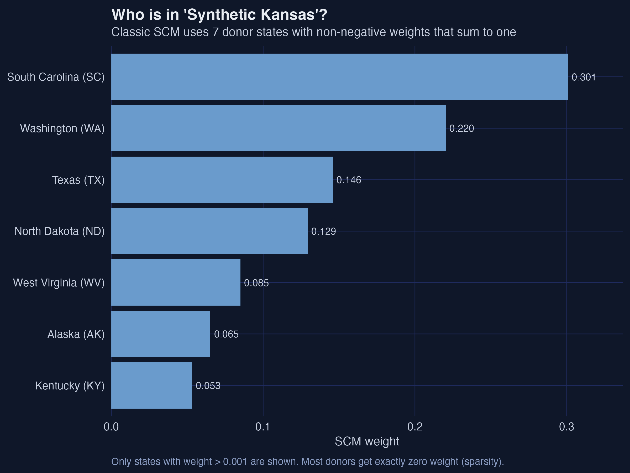
SCM’s virtue is sparsity: 7 donors, 42 zeros, a recipe you can name

Donor weights for synthetic Kansas: South Carolina 0.30, Washington 0.22, Texas 0.15, North Dakota 0.13, West Virginia 0.09, Alaska 0.07, Kentucky 0.05.

42 of the 49 donors get exactly zero weight — the simplex constraint pushes them there. The seven that remain form a recipe you can defend. The cost of that interpretability is rigidity: if no convex recipe matches Kansas, SCM cannot do better, and the leftover mismatch becomes bias.

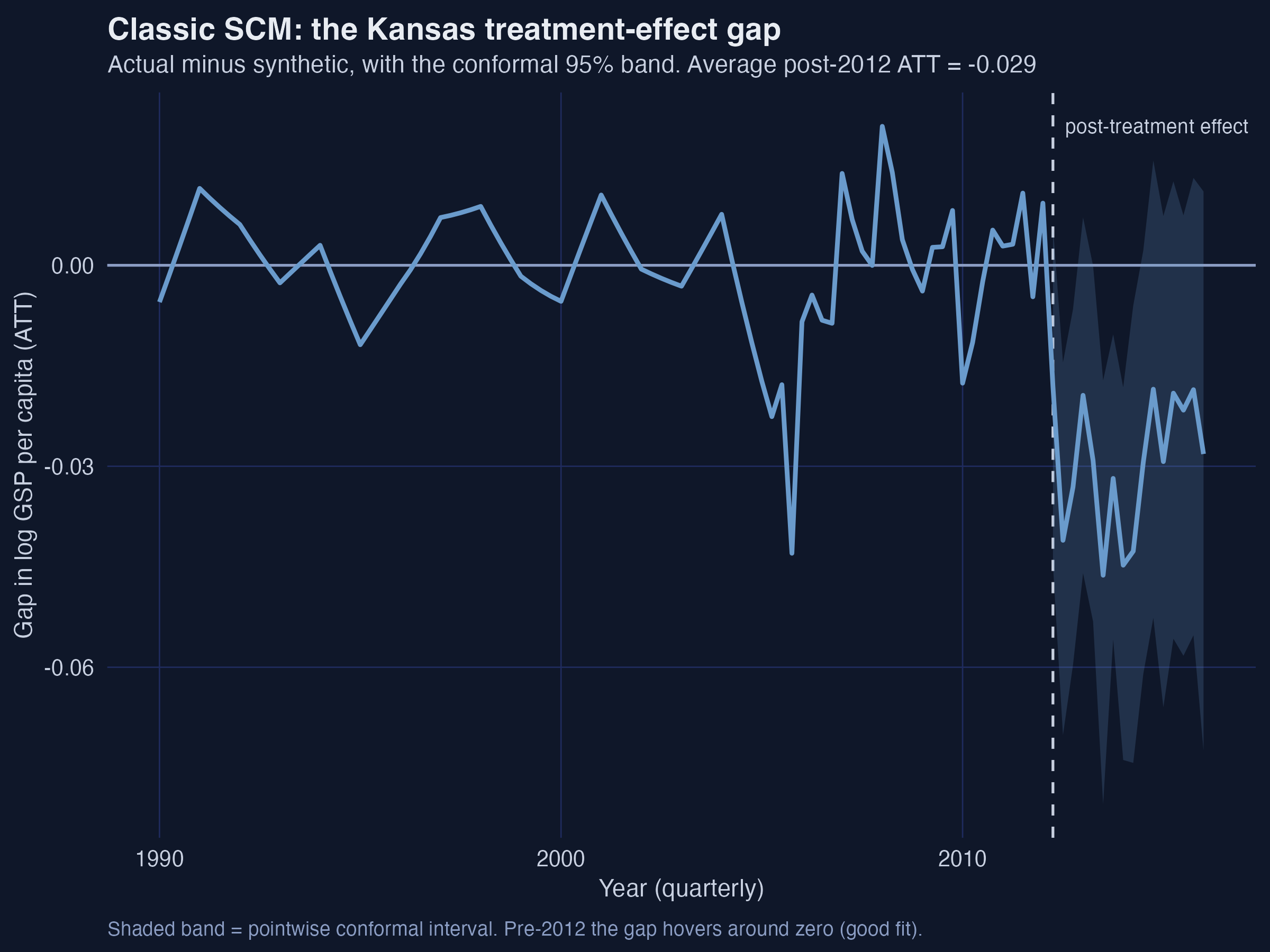
Classic SCM lands at −0.029, but the mid-2000s pre-fit leaks bias

The classic-SCM gap (actual − synthetic) with its conformal 95% band: near zero before 2012, persistently negative afterward.

Average post-2012 ATT = −0.0294 (≈ −2.9%), L2 imbalance 0.083 (79.5% better than uniform). But look at 2005–2006: a pre-treatment gap reaching −0.043, where the true effect is zero by definition. That’s pure imbalance — SCM simply could not match Kansas there. That stubborn bulge motivates everything that follows.

A −0.043 pre-treatment gap is bias hiding in plain sight

−0.043

worst pre-2012 quarter (2005 Q4) — as large as the effect itself, where the true effect is zero

This is the textbook trigger for augmentation. A convex combination cannot eliminate this gap; the leftover mismatch contaminates the post-treatment estimate. ASCM was built for exactly this regime.

ASCM estimates the leftover bias with an outcome model, then subtracts it

\[\hat{Y}_{1T}^{aug}(0) = \sum_i \hat{\gamma}_i^{scm} Y_{iT} + \Big( \hat{m}_{1T} - \sum_i \hat{\gamma}_i^{scm}\hat{m}_{iT} \Big)\]

Start from the plain SCM counterfactual (first term); add the imbalance the ridge outcome model \(\hat{m}\) predicts (the parenthesis). If the SCM fit were perfect, the correction vanishes — augmentation only acts where there is imbalance to fix.

The default outcome model is ridge regression of donors’ outcomes on their lagged outcomes. augsynth reports the parenthesis as “Avg Estimated Bias.” The estimator is doubly robust: it can also be read as “predict Kansas from the model, then correct with SCM-weighted donor residuals.”

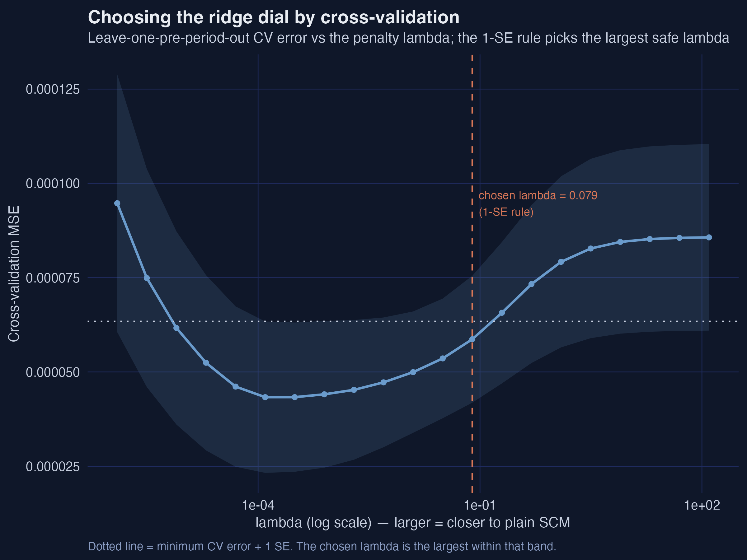
Cross-validation picks the penalty — the 1-SE rule keeps it conservative

Cross-validation MSE against the ridge penalty \(\lambda\) (log scale). The chosen \(\lambda = 0.079\) is the largest within one SE of the minimum.

Leave-one-pre-period-out CV. The curve is U-shaped; the one-standard-error rule deliberately picks the largest λ within one SE of the minimum — among indistinguishable choices, the one that keeps the augmented weights closest to the safe convex SCM solution. A smaller λ would chase fit at the cost of more extrapolation.

Augmentation deepens the effect to −0.040 and the bias is a third of it

−0.040

Ridge ASCM ATT (≈ −3.9%) · L2 falls 0.083 → 0.062 · estimated bias 0.011 ≈ ⅓ of the effect

Three numbers tell the story. The estimate deepens from −0.029 to −0.040 — augmentation reveals a larger effect. The pre-fit improves (L2 0.083 → 0.062, 84.7% better than uniform). And augsynth reports an estimated bias of 0.011, its own measure of how much imperfect matching distorted the SCM number — confirming the paper’s warning that poor fit understates the effect.

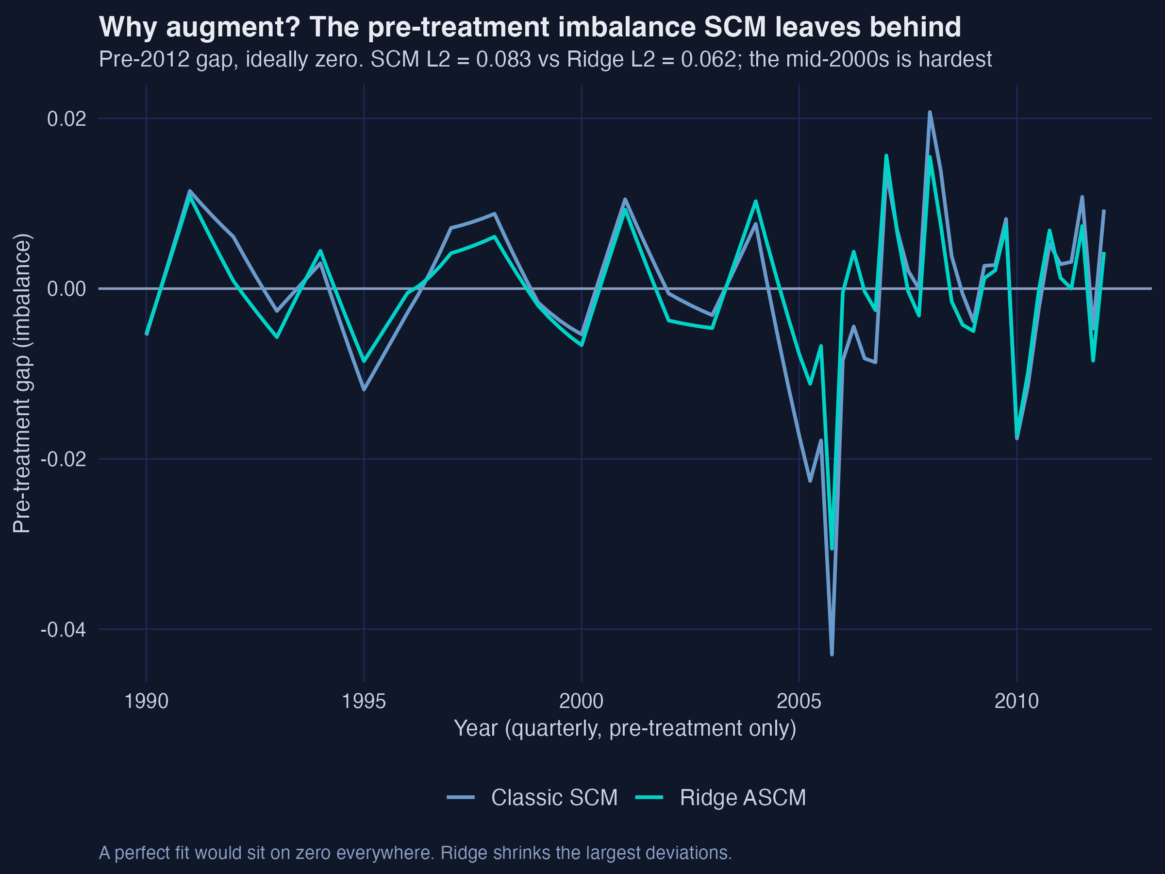
Ridge spent its budget exactly where SCM was failing — the mid-2000s

Pre-treatment imbalance, SCM vs Ridge ASCM. Ridge shrinks the largest deviations, pulling the 2005 Q4 gap from −0.043 to −0.031.

Restricting attention to the pre-period — where the gap should be zero — shows what augmentation fixed. SCM’s worst quarter (2005 Q4, −0.043) is pulled back to −0.031, and the rest of the turbulent mid-2000s is calmed. That is the bias correction at work, spent precisely where the convex hull broke down.

A better fit, but the same recipe: the weights barely move

Classic SCM

• convex weights only
• 7 donors, 42 exact zeros
• L2 imbalance 0.083
• ATT \(-0.029\)

Ridge ASCM

• penalized weights leave the simplex
• 21 small negative weights
• L2 imbalance 0.062
• ATT \(-0.040\) · RMS weight change just 0.015

Ridge ASCM is equivalent to a penalized SCM: it lets the weights leave the simplex but penalizes how far they stray from the trustworthy SCM solution. A large λ keeps them close; here the RMS change is only 0.0147 — almost nothing. Synthetic Kansas is essentially the same blend, bought a de-biased estimate for a tiny, principled departure from the convex hull.

Six lines fit Ridge ASCM in R — the formula mini-language does the work

syn  <- augsynth(lngdpcapita ~ treated, fips, year_qtr, kansas,
                 progfunc = "None",  scm = TRUE)   # classic SCM
asyn <- augsynth(lngdpcapita ~ treated, fips, year_qtr, kansas,
                 progfunc = "Ridge", scm = TRUE)   # CV picks lambda
summary(asyn)                # avg ATT, L2 imbalance, est. bias
plot(asyn)                   # gap with a conformal 95% band

The whole augmentation is one keyword: progfunc = “Ridge” instead of “None.” Cross-validation chooses λ automatically. summary() prints the average ATT, the L2 imbalance, and the estimated bias; the full ggplot pipeline lives in analysis.R.

Add six covariates and balance gets near-perfect; the effect deepens to −0.061

Specification	ATT (log pts)	≈ % effect	Pre-fit L2	Est. bias
Classic SCM	−0.029	−2.9%	0.083	—
Ridge ASCM	−0.040	−3.9%	0.062	0.011
Covariate ASCM	−0.061	−5.9%	0.054	0.027

The more we de-bias and balance, the larger the measured damage — the un-augmented SCM number is the conservative one.

Adding revenue, wages, establishments and employment after the | drives covariate imbalance to 0.005 (97.7% better than uniform). Fixed-effect (−0.034) and residualized (−0.055) variants fall between these. Every route agrees on sign and rough size — that monotonic pattern is reassuring, not alarming.

The Resolution

Act III

The headline: a persistent ~3.9% GDP shortfall, de-biased

−0.040

Ridge ASCM ATT · strongest in 2013–2014 · robust in sign across all five specifications

Between the no-controls baseline (−0.029) and the kitchen-sink covariate fit (−0.061), the principled Ridge default lands at −0.040 off the same interpretable recipe. The supply-side promise of accelerated growth simply does not appear in the data.

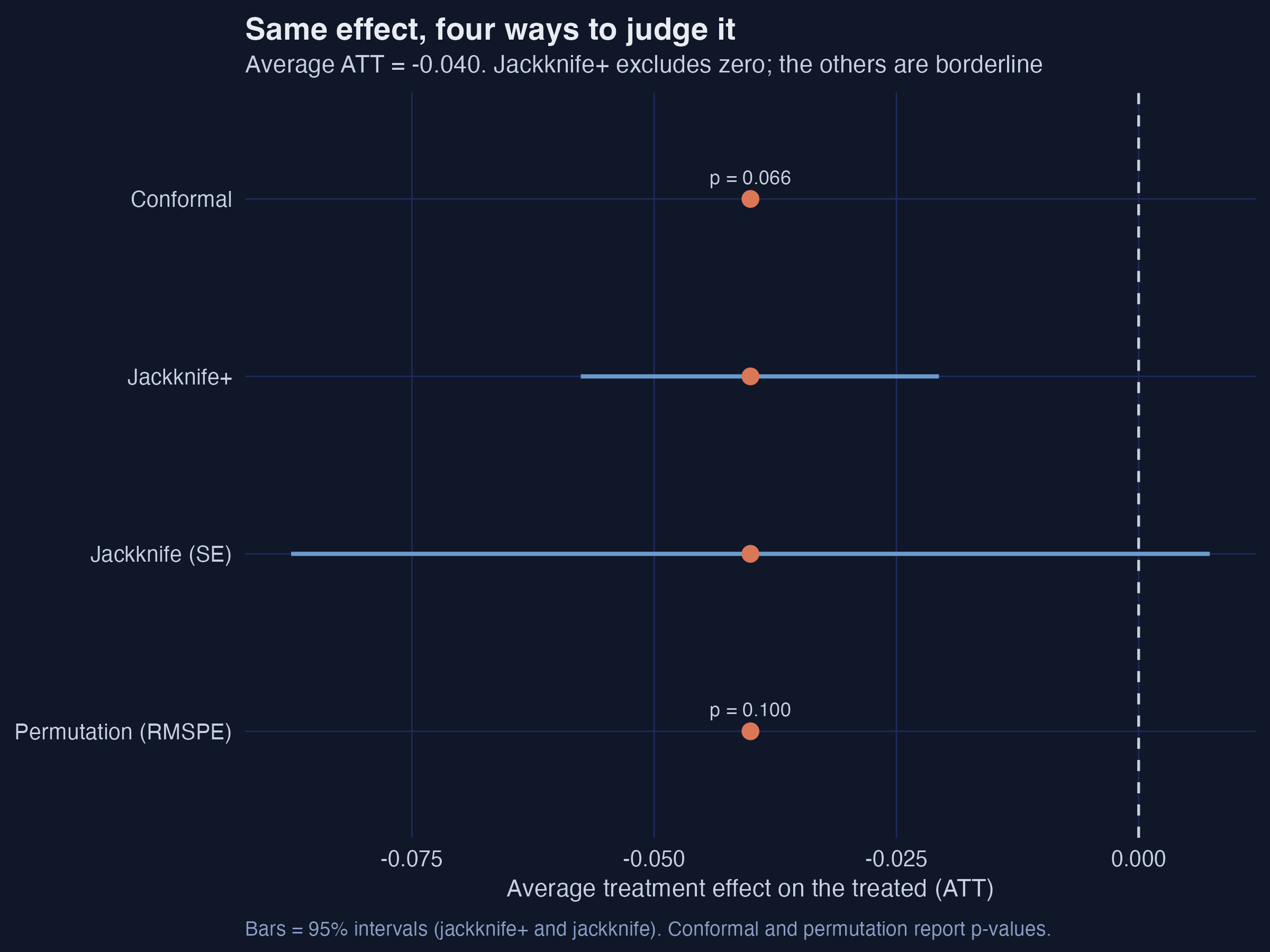
Same point estimate, four verdicts: significance depends on the question

Four inference methods side by side. All share the −0.040 estimate; jackknife+ excludes zero, while conformal (p = 0.066), permutation (p = 0.10), and the leave-one-donor jackknife are borderline.

The lesson of the section in one figure. The point estimate is −0.040 in all four; only the uncertainty differs. They probe different variation — over time (conformal, jackknife+) vs over units (permutation, leave-one-donor jackknife). Jackknife+ CI [−0.058, −0.021] excludes zero; conformal p = 0.066; permutation ranks Kansas 5th of 50 (p = 0.10); the leave-one-donor jackknife Wald CI [−0.088, 0.007] includes zero because South Carolina alone is 30% of the blend. Reporting all four is more honest than cherry-picking 0.05.

Does LASSO-style selection make this causal? No — the assumptions still carry it

Objection. Augmentation just de-biases the fit; it can’t manufacture identification.

Response. Correct. ASCM disciplines selection; it cannot manufacture identification. The ATT still needs a credible donor blend, no anticipation, no interference — and the gap mixes the tax cut with the drought and aerospace shocks. Suggestive-to-moderate evidence, not a knock-down result.

Steelman, don’t strawman. The ATT is identified only if a weighted donor blend can stand in for Kansas’s untreated path, with no anticipation and no interference; ASCM improves the counterfactual but does not relax those identifying assumptions. Significance is genuinely borderline, and the estimate is the net gap — it cannot strip out the 2012–2013 drought or the aerospace-sector shocks a synthetic control cannot separate.

The better we make the comparison, the worse the tax cut looks — and never good.

The single takeaway. Across SCM → Ridge → covariate the estimate moves −0.029 → −0.040 → −0.061; at no point does the supply-side experiment look successful. The un-augmented SCM number was the conservative one, understating the effect because of the very imbalance ASCM was built to remove.