Synthetic Control in R

What did conflict cost the Basque Country? A counterfactual built from data

−0.580ATT · thousand 1986 USD/capita

2 of 16active donors · 85% Catalonia

2 of 8placebo rank · pseudo p = 0.25

Carlos Mendez

Nagoya University (GSID)

June 11, 2026

The Tension

Act I

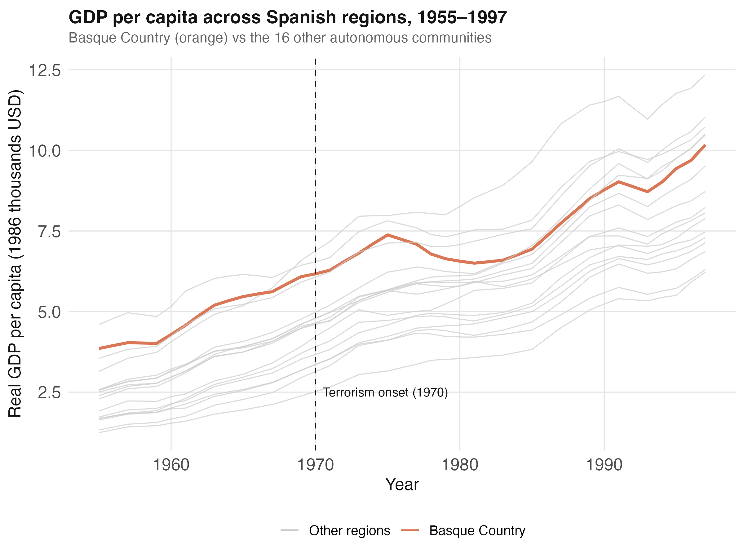
We never see the Basque economy without the conflict

In 1970 the Basque Country entered decades of sustained terrorist activity. The natural question — what did it cost? — has no easy answer.

The path we observed is only half the story. The path without conflict — the counterfactual — was never recorded. How do you measure a road not taken?

This is the fundamental problem of causal inference in a single case study. We observe one Basque Country with conflict; we never observe the parallel-universe Basque without it. Classical difference-in-differences needs many treated units; here there is exactly one. That is what motivates synthetic control.

One treated region, no clean comparison — until we build one

GDP per capita across Spanish regions, 1955–1997. The Basque Country (orange) sits among the richest regions throughout — so no single region is a clean comparison.

The spoiler figure for the data structure. Don’t over-explain: just plant that the Basque (orange) is consistently one of the richest regions, near the top of the distribution. A weighted average of poorer regions cannot reproduce its level — so the optimizer will have to load heavily on the few comparably wealthy, industrial regions. We come back to this when Catalonia and Madrid emerge as the only two donors.

Where we’re going

• The single-treated-unit problem — why difference-in-differences breaks
• The recipe: a weighted blend of donor regions matched on pre-1970 fit
• The headline gap — actual minus synthetic Basque (the ATT)
• Two falsification tests: a Catalonia placebo and an in-space placebo

The Investigation

Act II

The estimand is the ATT: the gap from the counterfactual we never see

\[\alpha_{1t} = Y_{1t} - Y_{1t}^{N}, \quad t \geq 1970\]

Treatment effect = actual GDP minus the no-conflict counterfactual \(Y_{1t}^{N}\).

The fundamental problem: \(Y_{1t}^{N}\) is never observed. Synthetic control estimates it as a weighted average of donor regions.

State the estimand explicitly: the average treatment effect on the treated, year by year. Y₁ₜ is realized; Y₁ₜ^N is the missing potential outcome. Everything in the method is machinery to estimate that one unobserved quantity credibly.

The estimator replaces the counterfactual with a weighted donor recipe

\[\hat{\alpha}_{1t} = Y_{1t} - \sum_{j=2}^{18} w_j^{*}\, Y_{jt}, \quad t \geq 1970\]

The donor weights \(w_j^{*}\) are non-negative, sum to one, and are picked to match the Basque pre-treatment predictors.

If the pre-1970 match is good, the post-1970 gap is the most plausible estimate of the conflict’s cost.

The estimator is the actual outcome minus the synthetic outcome. The synthetic is a convex combination of the 16 donor regions. The identifying logic: match the observables before treatment, and — under the factor-model assumptions of Abadie et al. — the unobservable counterfactual is matched too.

The lab: 18 regions, 43 years, 13 predictors, treatment in 1970

• Outcome — gdpcap, real GDP per capita in 1986 thousand USD
• Treated unit — the Basque Country (region 17), conflict onset 1970
• Donor pool — the 16 other Spanish autonomous communities
• Predictors — 13 covariates: education, investment, sector shares, density

774 rows = 18 regions × 43 years. Pre-treatment window 1955–1969; post-treatment evaluation 1970–1997.

The basque panel ships with the Synth package. Region 1 is the Spanish national aggregate, which we drop. The pre-treatment outcomes Z are annual GDP over 1960–1969; the predictors X are the 13 matched covariates. Keep this slide as the orientation map for the whole method.

Two nested optimizations: inner picks the recipe, outer picks what matters

\[W^{*}(V) = \arg\min_{W \in \mathcal{W}} \lVert X_{1} - X_{0}W \rVert_{V}\]

The inner problem finds donor weights \(W\) matching the treated predictor profile \(X_1\), measured in a \(V\)-weighted norm.

\[V^{*} = \arg\min_{V} \, (Z_{1} - Z_{0}W^{*}(V))'(Z_{1} - Z_{0}W^{*}(V))\]

The outer problem picks predictor weights \(V\) so the induced recipe minimizes pre-1970 outcome error.

Every candidate V requires solving the inner W problem first — a nested optimization. V acts as importance dials on the predictors: match the saffron exactly, the salt can be approximate. synth() uses BFGS for the outer search and a constrained quadratic program (kernlab) for the inner one. Don’t dwell on the algebra; convey that the algorithm both blends donors and decides which predictors deserve weight.

dataprep() then synth() — the whole estimation is two calls

basque_dp <- prepare_basque(treated_id  = 17,
                            control_ids = c(2:16, 18))   # 16-region donor pool

run_synth_quiet <- function(dp)
  synth(data.prep.obj = dp, optimxmethod = "BFGS", verbose = FALSE)
basque_synth <- run_synth_quiet(basque_dp)

basque_synth$solution.w        # the donor weights W*

prepare_basque() is a helper wrapping dataprep() that packages the four matrices X1, X0, Z1, Z0 and parameterizes the treated unit and donor pool — which makes the placebo exercises trivial later (just change treated_id). synth() runs the nested optimization. The full helper lives in analysis.R; here we show the load-bearing calls.

The optimizer keeps just 2 of 16 donors — a sparse, readable recipe

Diagnostic	Value
W weights sum to	1
Active donors (\(w > 0.01\))	2 of 16
Pre-treatment loss \(V\)	0.0089
Pre-treatment loss \(W\) (MSPE)	0.2467

Sparsity is typical: few donors resemble the treated unit, the rest get zero.

Three numbers tell the story. The weights sum to one (convexity respected). Only 2 of 16 donors get non-trivial weight. Both pre-treatment losses are small — a tight fit. This sparse solution is one of synthetic control’s appeals over black-box prediction: you can read the recipe.

The synthetic Basque is 85% Catalonia and 15% Madrid

Region	Weight
Cataluna	0.851
Madrid (Comunidad De)	0.149
Every other region	0

Basque \(\approx\) 85% Catalonia + 15% Madrid — the only two comparably industrial, urban, wealthy regions.

This is the one-line summary a reader can carry away. Catalonia and Madrid are the only pre-1970 Spanish regions comparably industrial and wealthy, so the optimizer leans entirely on them. Remember Catalonia’s 85% dominance — it returns as a caveat in Act III’s placebo. The dataset stores the region as “Cataluna” without the tilde.

The match is excellent where it matters — pre-1970 GDP and education

Predictor	Treated	Synthetic	Donor mean
Pre-1970 GDP/capita	5.28	5.27	3.58
School (primary) %	85.9	82.3	80.9
Industry share %	45.1	37.6	22.4
Agriculture share %	6.84	6.18	21.4
Pop. density 1969	247	196	99.4

Outcome-relevant predictors match closely; density is the largest gap.

Pre-treatment GDP matches almost exactly: 5.28 vs 5.27, against a donor mean of just 3.58 — the synthetic is far closer to Basque than the average region is. Education shares fall within a few points. The optimizer correctly recognized Basque as an industrial, low-agriculture region (agriculture 6.84% vs donor mean 21.4%) and downweighted farming economies. Density (247 vs 196) is the largest gap but it is a static control, not an outcome predictor, so it carries little weight in the fit.

The Resolution

Act III

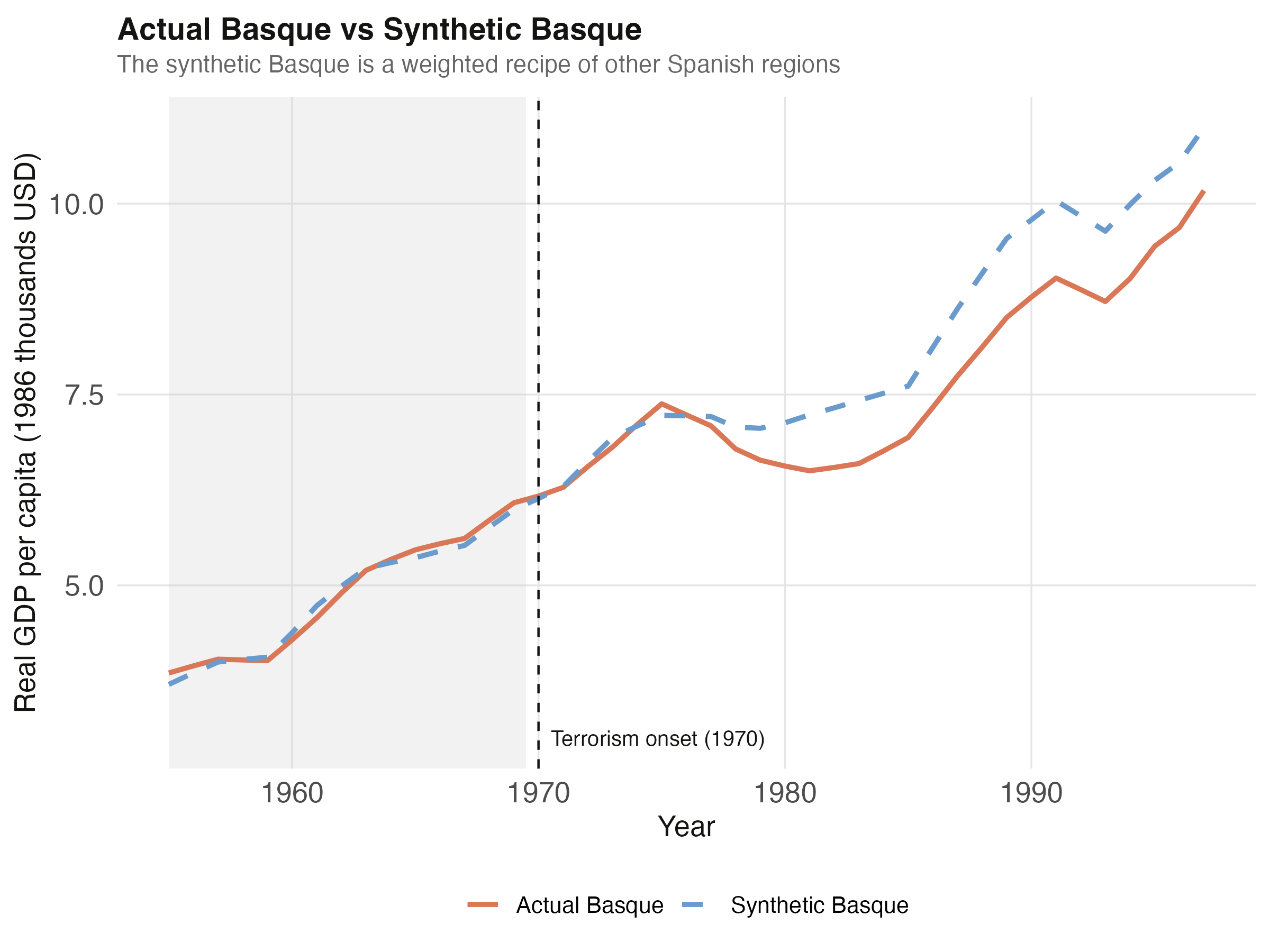
Before 1970 the lines are one; after 1970 they split apart

Actual Basque (orange) vs synthetic Basque (blue dashed). Pre-treatment window 1955–1969 shaded; the vertical line marks conflict onset in 1970.

Walk the audience along the two lines. Pre-1970 they are nearly indistinguishable — both climb from about 3.8 to 6.2 thousand USD. After 1970 they diverge: the synthetic keeps climbing toward 11 thousand by 1997 while the actual Basque stalls through the 1980s and recovers only to 10.2. The widening orange-vs-blue band is the visual signature of the conflict’s cost.

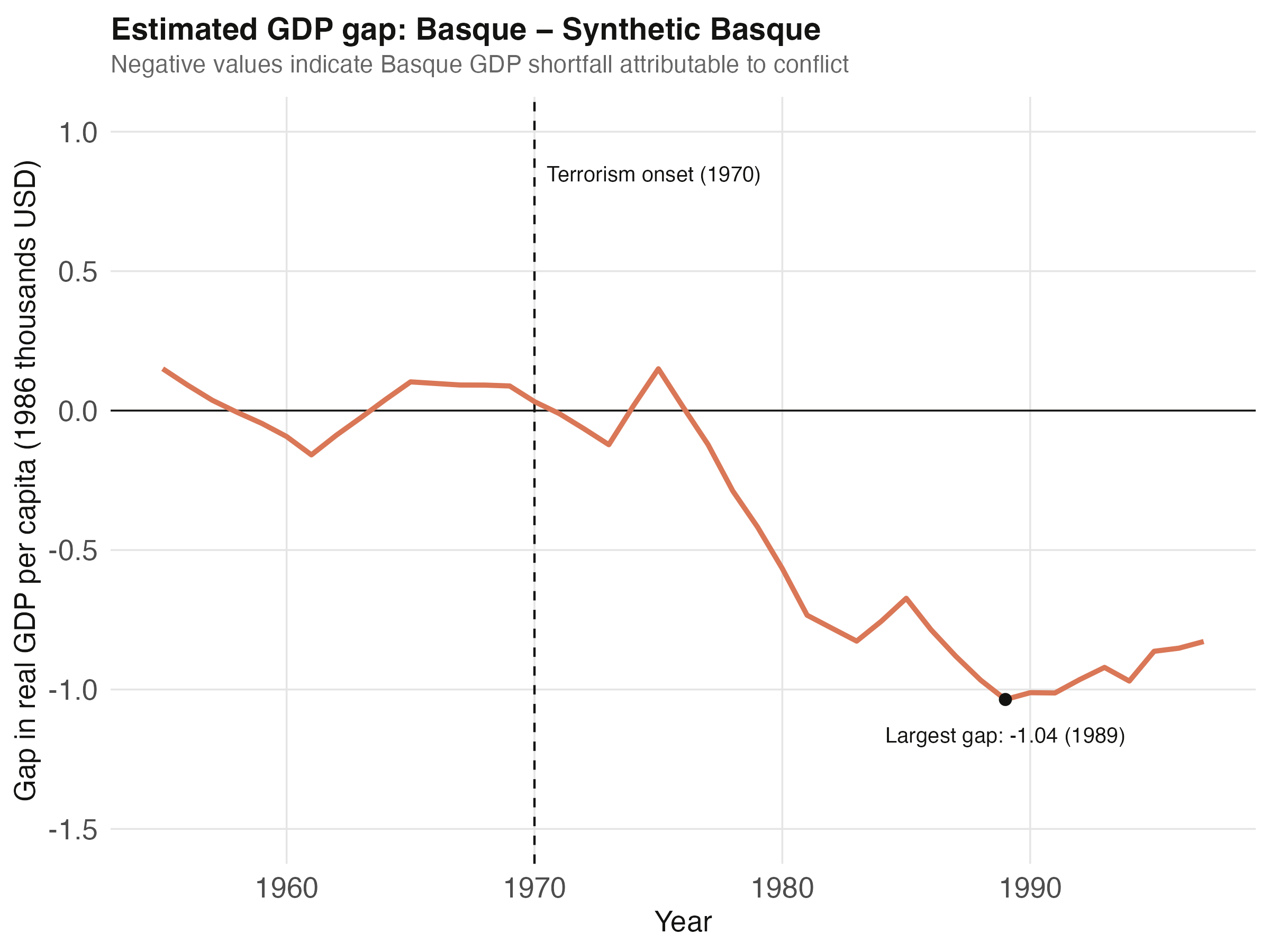
The gap is the cost — peaking at −1.04 thousand USD in 1989

Estimated GDP gap (Basque minus synthetic Basque). Essentially zero before 1970, then negative — the deepest deficit of −1.04 thousand USD falls in 1989.

The gap series makes the divergence quantitative. It is essentially zero from 1955 to 1970 — another way of seeing the good pre-treatment fit. After 1970 it turns negative and bottoms at −1.036 thousand USD per capita in 1989 before partially recovering. Averaging from 1970 on gives the headline ATT.

The conflict cost the Basque Country −0.580 thousand USD per capita per year

−0.580

\(\widehat{\mathrm{ATT}}\), average 1970–1997 (thousand 1986 USD/capita) · roughly an 8% income shortfall

The headline causal estimate. Average Basque GDP over the window was about 7 thousand USD, so a 0.58 shortfall is roughly 8% of the counterfactual income the region would have generated. Large in absolute terms and consistent with the narrative that sustained conflict discouraged investment, talent retention, and tourism.

A single placebo isn’t enough — Catalonia’s ratio is nearly as big

Catalonia placebo	Value
Pre-1970 MSPE	0.006
Post-1970 MSPE	0.391
Post/pre ratio	64.7

Comparable to Basque’s own ratio of 60.1 — one placebo run has limited inferential power.

The first falsification pretends Catalonia — a never-treated donor — was the treated unit. Its pre-1970 MSPE is tiny (0.006) but post-1970 MSPE is large (0.391), a ratio of 64.7. That is comparable to Basque’s 60.1, which is uncomfortable at first glance. The honest answer: a single placebo says little; we need the full distribution across all regions, which the in-space placebo provides.

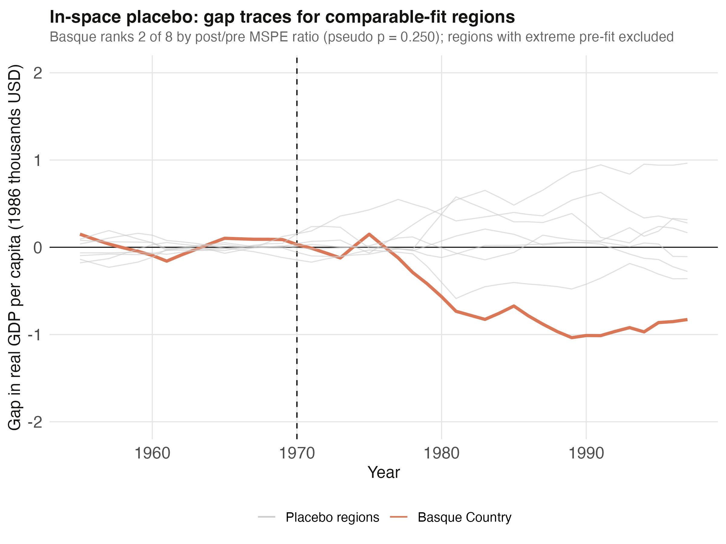
In the comparable-fit placebos, the Basque ranks 2 of 8

In-space placebo gap traces for the 8 comparable-fit regions. The Basque (orange) ranks 2 of 8 by post/pre MSPE ratio — at the loud edge of the chorus, not far outside it.

The full in-space placebo runs the pipeline 17 times, once per treated region, then ranks the post/pre MSPE ratio. The raw rank (7 of 17) is misleading because tiny-pre-MSPE regions get astronomical ratios. Trimming to regions whose pre-fit is within a factor of 5 of Basque’s leaves 8 comparable regions; Basque ranks 2 of 8 (pseudo p = 0.250). The top spot goes to Catalonia — the same region that is 85% of the synthetic recipe.

The placebo is suggestive, not decisive — read it with the donor weights

Objection. If Catalonia tops the placebo ranking and is also 85% of the synthetic recipe, isn’t the Basque “effect” just the same Spanish industrial transition?

Response. A fair caveat. When a synthetic is built from one dominant donor, that donor naturally scores high in its own placebo — it has no close substitute to rebuild it. The result is consistent with a sizeable cost (rank 2 of 8, an 8% shortfall) but the small 16-region pool limits resolution (smallest pseudo p = 0.125). Report placebo and donor weights together, not separately.

Steelman, don’t strawman. The placebo evidence does not isolate the Basque effect from the broader industrial transition that affected Catalonia too. With only 16 donors the discrete pseudo-p cannot clear conventional thresholds. The structural point — dominant donors top their own placebos — is a feature of the method, and the lesson is to interpret the two diagnostics jointly.

Match the pre-treatment, build the counterfactual, read the gap.

The single takeaway. Synthetic control turns an unanswerable single-case question into a disciplined estimate: assemble a donor recipe that mimics the treated unit before treatment, let it run as the counterfactual, and read the post-treatment gap as the cost. For confidence intervals see the scpi package; for many treated units see generalized synthetic control.