Six Ways to Evaluate a Policy

Comparative case studies of California’s Proposition 99, in R

−18.9synthetic-control ATT (packs/capita)

+4.5ARIMA sign flip · same data

0.026placebo Fisher exact p

Carlos Mendez

Nagoya University (GSID)

June 11, 2026

The Tension

Act I

California’s smoking fell 48% after Proposition 99 — but how much was the tax?

In January 1989 California raised its cigarette tax by 25 cents. Per-capita sales fell from 116 packs (1970–1988) to 60 packs (1989–2000).

But the whole country was smoking less. How much of California’s drop did the policy actually cause?

This is the motivating puzzle. The raw 47.9% within-state drop bundles together the policy effect and the nationwide secular decline in smoking. Every method in this deck is an attempt to separate the two by building a counterfactual: what California would have done without the tax.

One dataset, six estimators — and they disagree from −28 to +4.5 packs

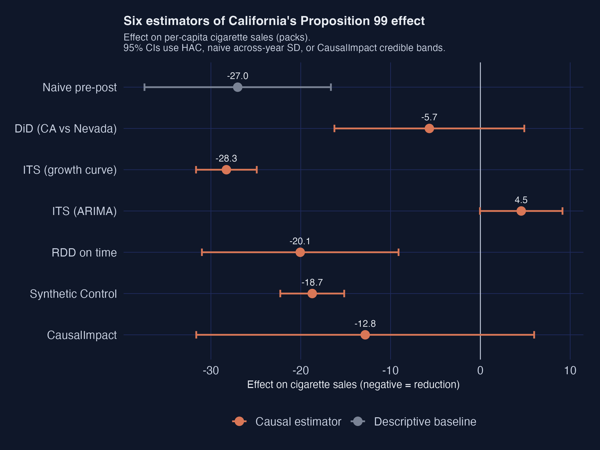
Effect on per-capita cigarette sales, 95% intervals · naive, DiD, two ITS, RDD-on-time, synthetic control, CausalImpact. Dashed line = zero.

The spoiler figure. Do not explain every row yet — just plant that one dataset fed to six estimator families produces answers ranging from −28 packs to a positive +4.5. The disagreement is the lesson. We earn each estimate in Act II and return to this plot in Act III.

Where we’re going

• The estimand: every method targets the ATT on California, 1989–2000
• Each method imputes the same missing piece — California’s no-policy counterfactual
• Six estimators, escalating discipline: naive · DiD · ITS · RDD · synthetic control · CausalImpact
• The lesson: the choice of counterfactual, not the data, drives the estimate

The Investigation

Act II

Causal inference is a missing-data problem: we never see \(Y(0)\) for treated California

\[Y_{it} = D_{it}\, Y_{it}(1) + (1 - D_{it})\, Y_{it}(0)\]

Each state-year has two potential outcomes; we observe only one. For California after 1989 the missing one is \(Y_{it}(0)\) — sales without the tax.

Every estimator in this deck is a different way to impute that missing \(Y_{it}(0)\).

Neyman–Rubin potential outcomes. D = 1 for California from 1989 onward, 0 everywhere else. The fundamental problem of causal inference (Holland 1986): for any treated unit we see at most one potential outcome. The whole tutorial is a tour of methods that fill in the missing Y(0).

The target is the ATT on California, not the population-wide ATE

\[\text{ATT} = \mathbb{E}\big[Y_{it}(1) - Y_{it}(0) \,\big|\, D_{it} = 1\big]\]

ATT (our target)

• effect on the unit actually treated
• California, post-1989
• identifiable with one treated unit

ATE (not estimable here)

• effect averaged over every state
• needs policy variation we lack
• Prop 99 was never randomized

Estimand discipline: name the causal quantity before quoting a number. ATT and ATE coincide only under constant treatment effects. With a single treated unit and a one-shot policy, the ATT on California is the only thing we can credibly target.

The shared logic: effect = observed − counterfactual; only the counterfactual differs

Fixed for everyone

• California’s observed post-1989 series
• the policy date (1989)
• the 39-state panel

What each method changes

• naive → California’s pre-mean
• DiD → Nevada’s pre→post change
• ITS → California’s own pre-trend
• SCM → weighted donor blend
• CausalImpact → Bayesian fit on donors

Six dashed arrows feed one counterfactual box; the gap to the observed series is the effect.

This is the §1 Mermaid diagram re-expressed as two columns (revealjs does not bundle mermaid.js). The orange box — California observed — is identical across methods. The blue counterfactual box is the construction. Methods differ only in the data source feeding that construction and the identifying assumption it leans on.

Naive pre-post overstates the effect at −27 packs — it has no counterfactual at all

Quantity	Estimate	HAC SE	\(p\)
Pre-period mean (1984–88)	98.98	—	—
Post-period shift	−27.02	5.30	<0.001

Estimand: purely descriptive. Identifying assumption: California’s pre-level would have frozen — almost certainly false.

Method 1. Imputes Y(0) as California’s own pre-period mean. The −27.02 drop silently bundles the nationwide secular decline into the “effect”. It is the largest number any method reports — that is the warning sign, not a feature. It sets the upper bound the disciplined methods will shrink.

DiD against Nevada collapses to −5.7 packs — a single bad control destroys the contrast

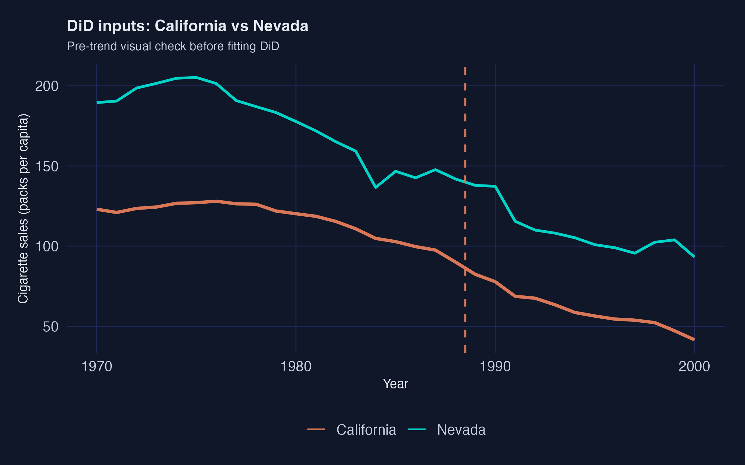
California (orange) vs Nevada (blue): both already falling before 1989, so the difference-in-differences contrast nearly vanishes.

Method 2. Estimand: ATT, identified by parallel trends with one neighbour. Nevada’s own sales fell 21.3 packs over the same window, so subtracting Nevada’s change from California’s leaves only −5.68 (p = 0.31), indistinguishable from zero. The textbook DiD pitfall: a single similar control subject to the same secular forces collapses the estimate. This motivates synthetic control.

ITS extrapolates California’s own pre-trend: a straight line gives −28 packs

\[\widehat{Y_{1t}(0)} = \hat\alpha + \hat\beta\, t, \qquad t > t^*\]

A linear fit on 1970–1988 (\(\hat\beta = -1.78\) packs/year, \(R^2 = 0.74\)) extended forward; the gap to observed averages −28.3 packs.

Assumption: the pre-trend has the right shape. No comparison unit — so it can’t separate policy from the secular decline.

Method 3a. ITS needs no control unit — it borrows from California’s own past — but pays in a stronger pre-trend assumption. −28.3 is essentially the naive −27.0 because both use only within-California information. Suggestive coincidence, not reassurance: both can be biased the same way.

Swap the line for an AICc-chosen ARIMA and the effect flips sign to +4.5 packs

+4.5

ITS via ARIMA(1,2,0) · the counterfactual bends below observed, implying the tax raised smoking

Method 3b. AICc selected ARIMA(1,2,0) — two rounds of differencing track the late-1980s acceleration and extrapolate it aggressively. The forecast lands below the observed post-period series, so the model concludes Prop 99 increased sales by 4.5 packs. Plainly wrong. The cautionary tale: AICc minimises in-sample fit, which can come from momentum that does not persist out-of-sample.

Why the ARIMA counterfactual misfires: it forecasts below what California actually did

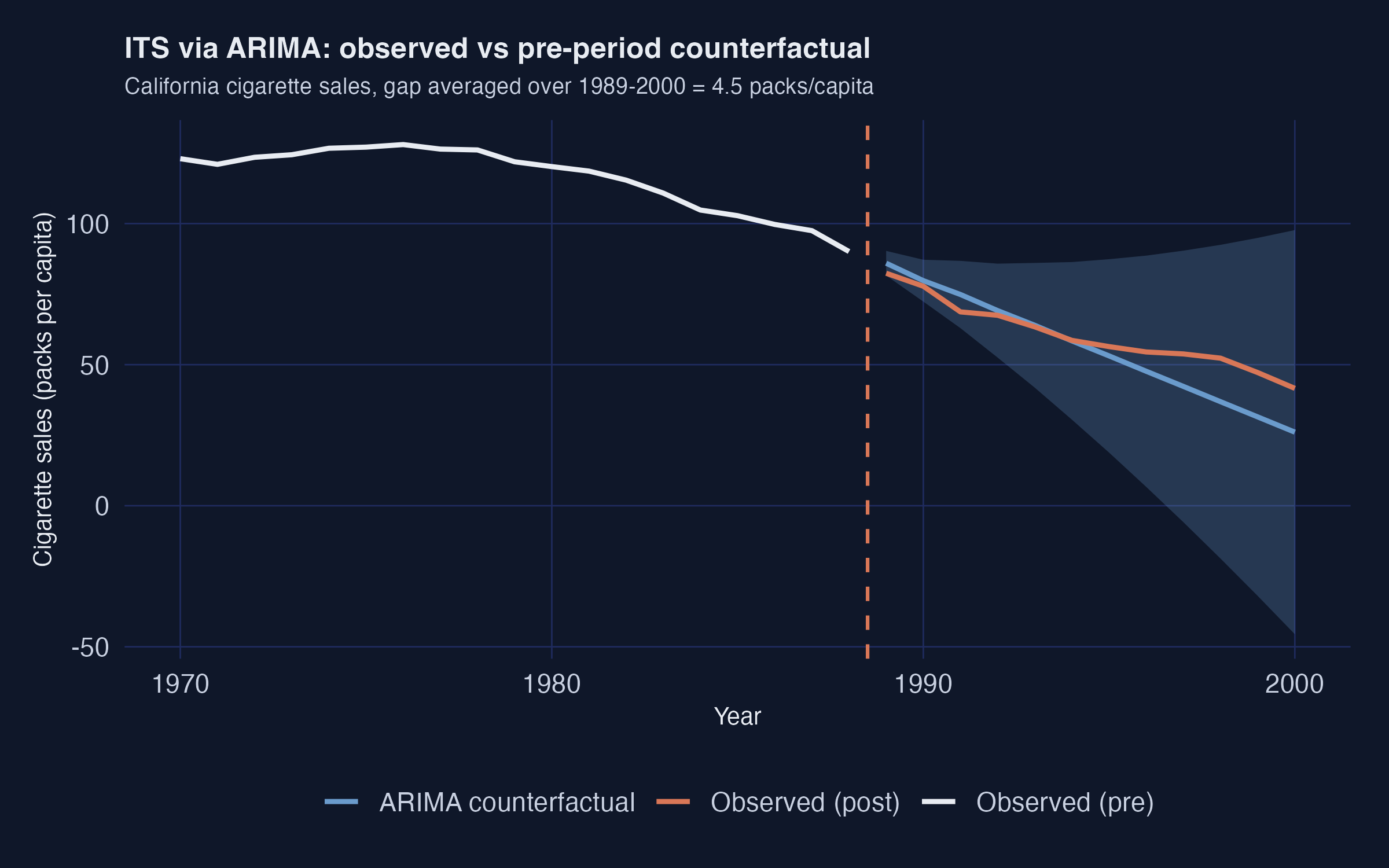
ARIMA(1,2,0) counterfactual (dashed, with 95% band) sits below the observed orange series throughout 1989–2000.

The visual diagnostic. The double-differencing extrapolates the steep 1985–1988 drop. The model predicts ~50 packs by 2000; California actually hit ~60, so the gap is positive. The lesson is not “ARIMA is bad” — it is that single-model ITS is fragile; always pair it against a comparison-unit method.

RDD-on-time finds a −20 pack level break right at 1989

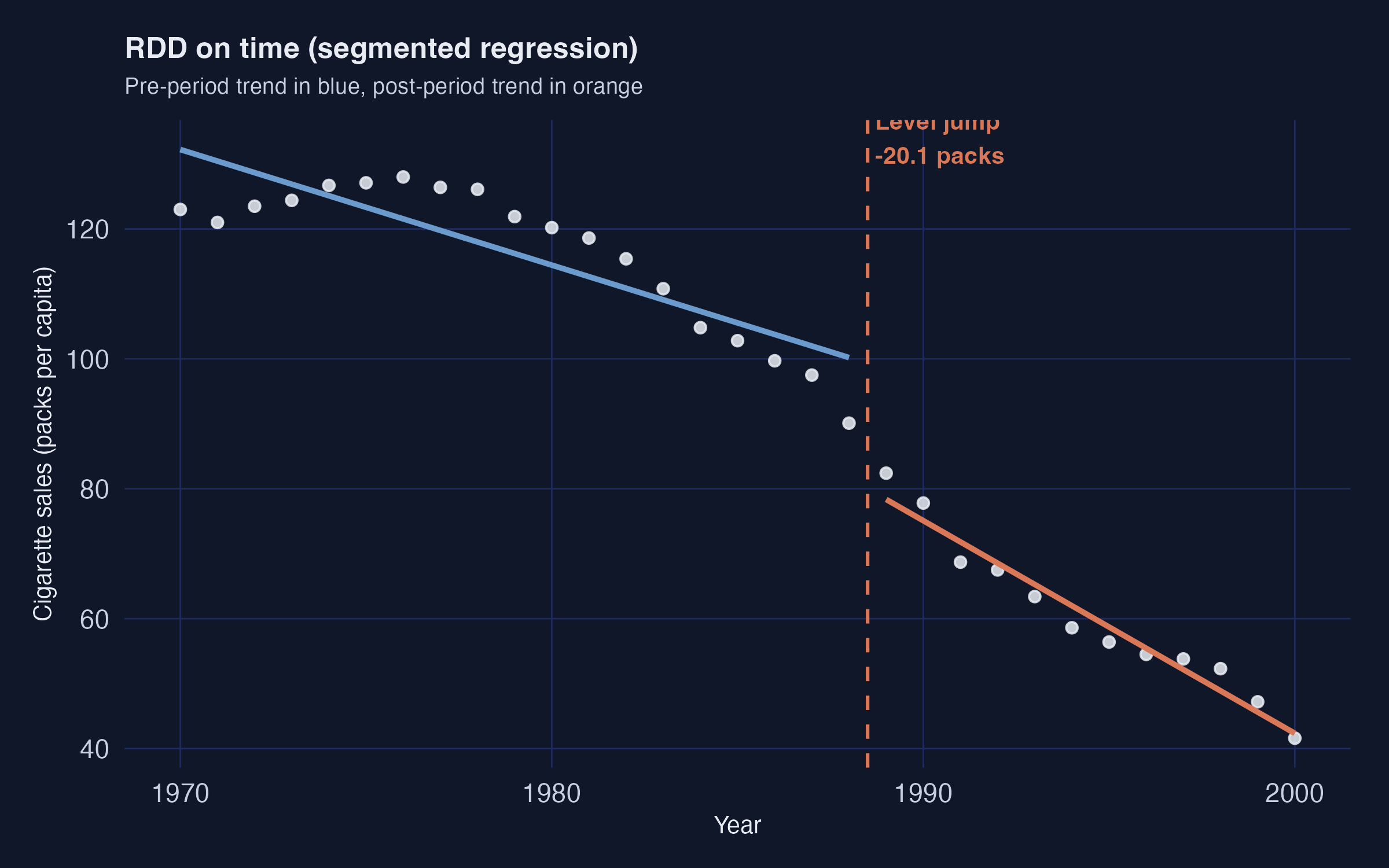
Piecewise pre/post linear fit (\(R^2 = 0.97\)): a clear level jump and a steeper slope at the 1989 threshold.

Method 4. Estimand: the level jump at the threshold. Identifying assumption: no other shock coincides with 1989. Level break = −20.06 packs (HAC SE 5.59, p = 0.001); the post slope steepens by an extra −1.49 packs/year. This is the first method to land in the credible −13 to −20 “consensus” range. Caveat: time-as-running-variable RDD inherits ITS’s pre-trend risk.

Synthetic control blends donors instead of picking one: −18.9 packs

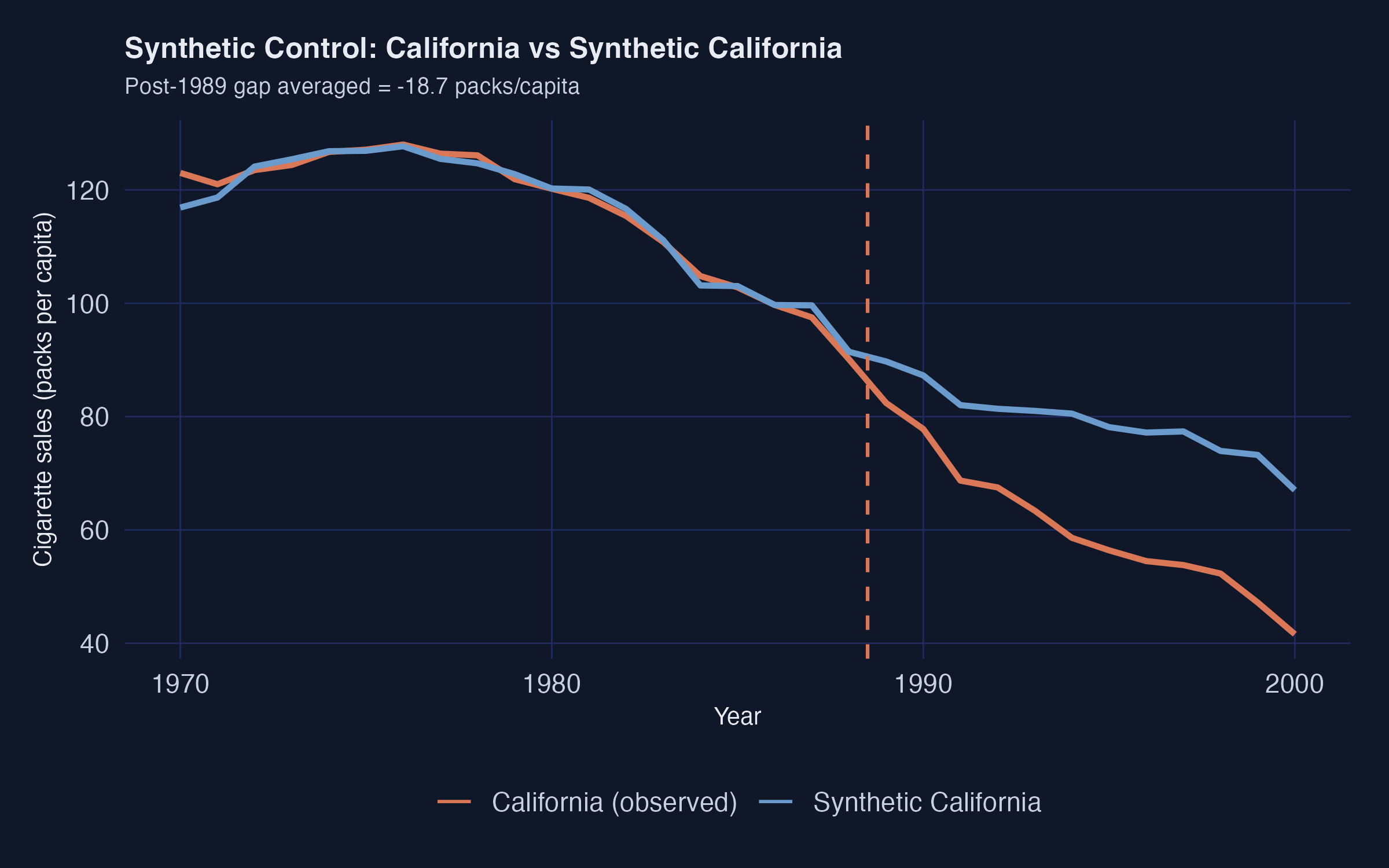
California (observed) vs synthetic California: near-perfect pre-1989 fit, then a gap opens and widens to ~30 packs by 2000.

Method 5. Estimand: ATT, identified by a convex donor combination matching the treated pre-period. Where DiD needed parallel trends with one neighbour, synthetic control needs them with a data-driven blend of many. The optimiser does the matching, so no hand-picked control. ATT = −18.85 packs, within rounding of Abadie et al. (2010). The pre-period fit is the credibility check.

Synthetic California is five states, anchored on lagged cigarette sales

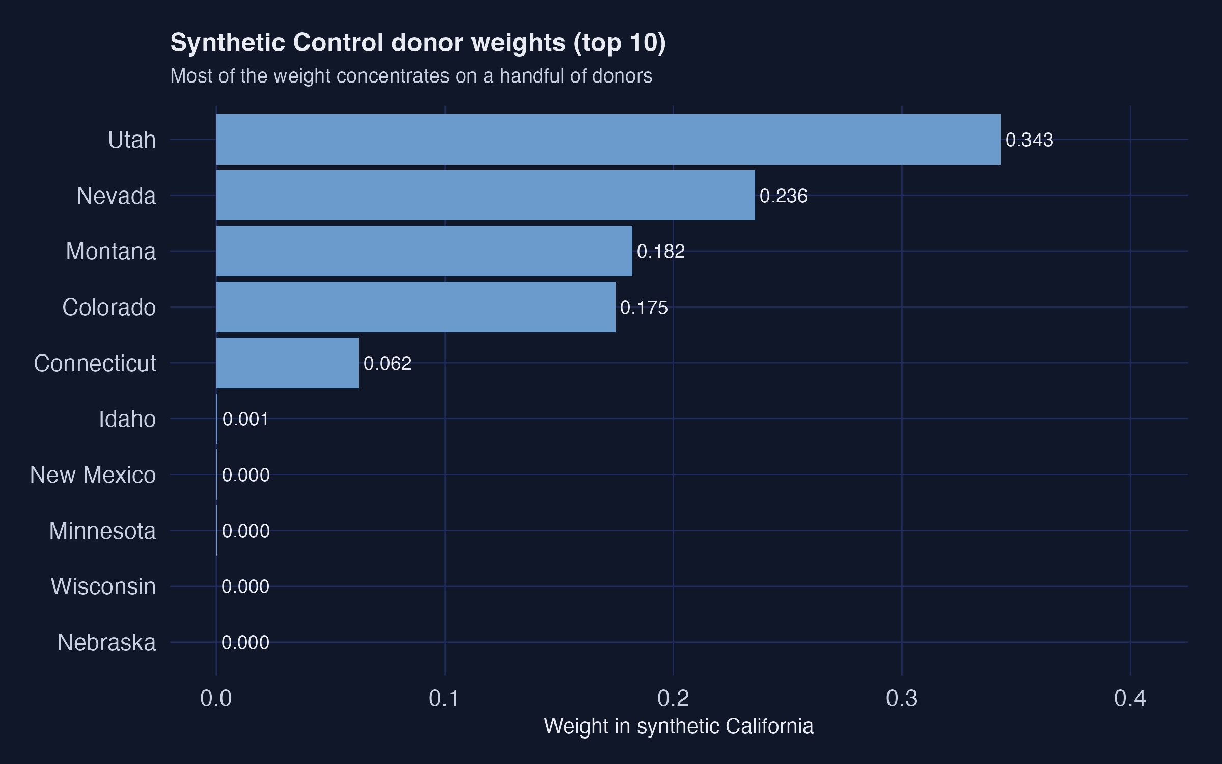
Faceted plot_weights output: five donor states carry ~100% of the weight (left); two lagged outcomes dominate the V matrix (right).

Utah 34%, Nevada 24%, Montana 21%, Colorado 15%, Connecticut 6% — every other state ~0. On the predictor side, cigsale_1975 (0.468) and cigsale_1980 (0.412) carry 88% of the V matrix. The optimiser decided: the best predictor of California’s cigarette sales is other states’ cigarette sales. Caution: V-weights are good-matching predictors, NOT a causal ranking.

Six lines fit synthetic control end-to-end with tidysynth

prop99_syn <- prop99 |>
  synthetic_control(outcome = cigsale, unit = state, time = year,
                    i_unit = "California", i_time = 1988,
                    generate_placebos = TRUE) |>
  generate_predictor(time_window = 1980, cigsale_1980 = cigsale) |>
  generate_weights(optimization_window = 1970:1988) |>
  generate_control()

The four-stage tidy pipeline: declare the treated unit and intervention time, define matching predictors (lagged outcomes plus covariates — abbreviated here), solve the constrained quadratic program for donor weights, then build synthetic California and the gap series. generate_placebos = TRUE also refits every donor as if treated, which powers the inference in the next slides.

The matching works: synthetic California nails the pre-period the donor average misses

Predictor	California	Synthetic	Donor avg
cigsale_1975	127.1	127.0	136.9
cigsale_1980	120.2	120.2	138.1
cigsale_1988	90.1	91.4	114.2

On 1988 sales, synthetic California (91.4) almost matches the real 90.1 — the donor average (114.2) is 24 packs off.

Balance table. Read the synthetic column against California: far closer than the unweighted donor average on every predictor. That 24-pack gap on cigsale_1988 between the donor average and California is exactly the bias the naive pre-post method silently absorbed. Good pre-period balance is what licenses reading the post-period gap as an effect.

Inference without a standard error: California ranks 1st of 39, Fisher exact \(p = 0.026\)

0.026

Placebo Fisher exact \(p\) · MSPE ratio 123.9, more than 2.5× the next-highest state

The right uncertainty for synthetic control is the placebo permutation, not a cross-year SD. Refit treating each donor as if treated, rank California’s MSPE ratio (post/pre). California is rank 1 of 39; p = 1/39 = 0.026. The MSPE ratio of 123.9 dwarfs Georgia’s 47.2. Under a null of no effect, a unit this extreme arises ~2.6% of the time.

CausalImpact hands the donors to a Bayesian model: −13 packs, 92% posterior probability

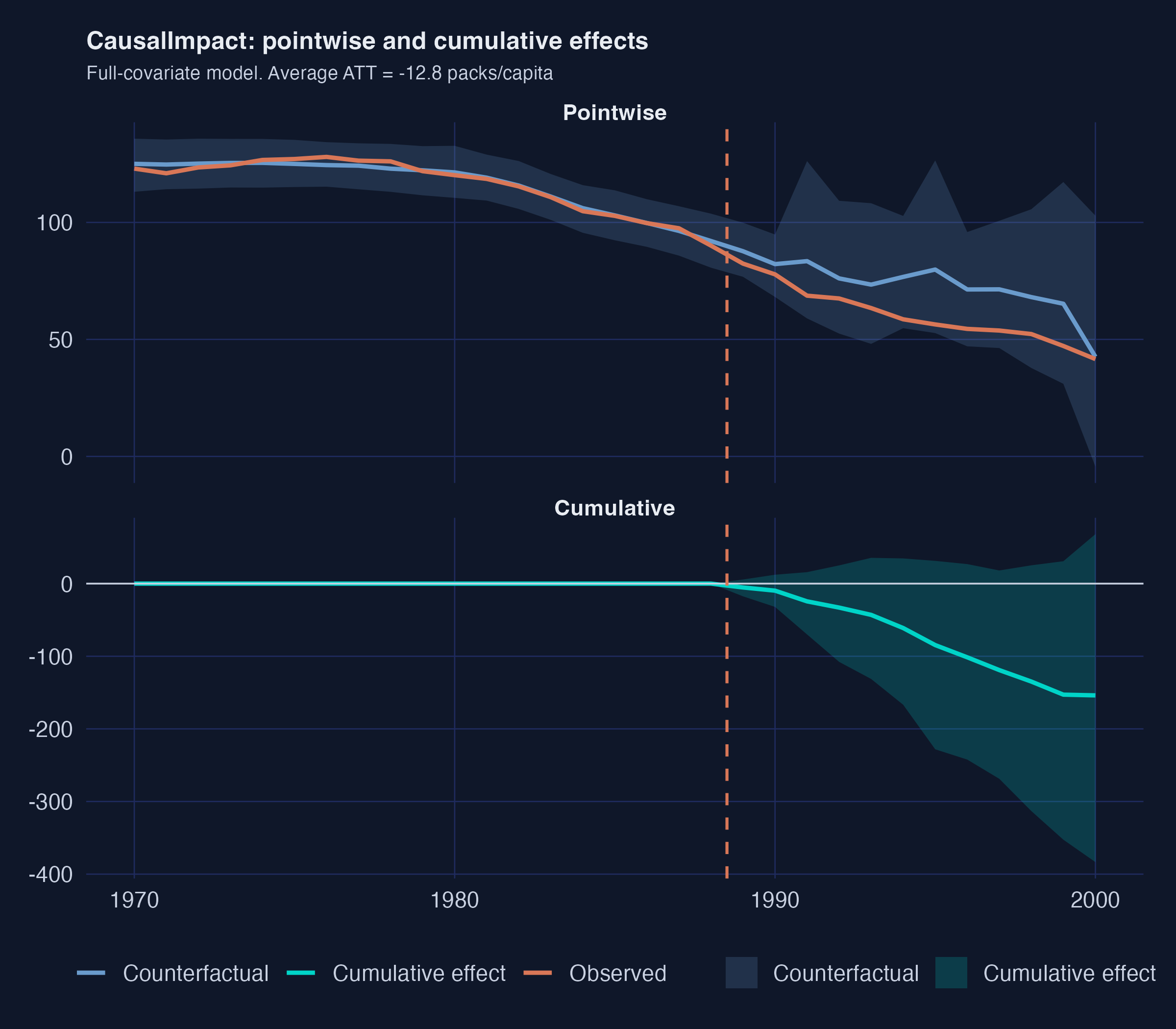
Top: observed California vs Bayesian counterfactual with a widening credible band. Bottom: cumulative effect reaching ~−150 packs by 2000.

Method 6. Estimand: ATT, identified by a BSTS prior plus a regression on donor series. Full-covariate model: −13 packs (95% CrI [−32, +5.7]), 92% posterior probability of an effect. Cigarette-only model strengthens to −21 packs, 97% probability. The only method here delivering a credible interval — a direct probability statement about the parameter — rather than a frequentist band.

The Resolution

Act III

Five of six methods converge on a 13–20 pack reduction — the disagreement is informative

Method	Estimand	Estimate
Naive pre-post	descriptive	−27.0
DiD vs Nevada	ATT	−5.7
ITS growth	post-gap	−28.3
ITS ARIMA	post-gap	+4.5
RDD on time	level jump	−20.1
Synthetic Control	ATT	−18.9
CausalImpact	ATT	−12.8

Consensus cluster (RDD, SCM, CausalImpact): −13 to −20. Outliers: DiD collapses, ARIMA flips.

Three clusters. (1) Causal consensus — RDD −20.1, SCM −18.9, CausalImpact −12.8 — all principled donor-information machinery, overlapping intervals. (2) Pre-trend-only overshoot — naive −27, ITS-growth −28, ~50% too large, no comparison unit. (3) Broken outliers in opposite directions — DiD vs Nevada and ITS-ARIMA. The honest headline: ~15–20 packs.

The synthetic-control ATT is −18.9 packs, robust where single comparisons fail

−18.9

ATT on California, 1989–2000 · Fisher exact \(p = 0.026\) · matches Abadie et al. (2010) within rounding

The Act-III payoff. Between the no-counterfactual naive −27 and the DiD collapse, the weighted-donor blend lands at a defensible −18.85, confirmed by a placebo p of 0.026. A state legislator’s honest answer: sales fell ~18 packs per capita more than they would have without the tax, bounds −13 to −22, cumulative ~150–250 fewer packs per Californian over 12 years.

Does machine-selected matching make this causal? No — assumptions still carry the weight

Objection. Synthetic control’s data-driven donor weighting manufactures the identification.

Response. It does not. The ATT is identified only if a convex donor combination tracks California’s no-policy path — a pre-trend assumption the placebo test stresses but cannot prove. Triangulating across six estimators discloses where each assumption breaks; it never relaxes them.

Steelman, don’t strawman. Synthetic control disciplines selection of the counterfactual; it cannot rule out a coincident 1989 shock or a non-convex true counterfactual. The cross-method comparison is a triangulation, not a proof. Prop 99 was not randomized, so every estimate is conditional on an identifying assumption.

The choice of counterfactual — not the data — is the design decision that moves the answer.

The single takeaway. The same 39-state panel yields −28 to +4.5 packs purely because each method assumes a different missing Y(0). Single comparisons are fragile; weighted donor combinations are robust; automated model selection is not your friend in ITS. Credible policy evaluation triangulates across estimators rather than trusting any one.