What Does TWFE Actually Do?

Manual demeaning, OLS, and the Frisch–Waugh–Lovell theorem

−0.055286same coefficient, two routes

3.05e−16max difference · machine epsilon

1,200150 countries × 8 periods

Carlos Mendez

Nagoya University (GSID)

June 11, 2026

The Tension

Act I

feols(y ~ x | id + time) gives you an answer — but what did it do to the data?

One line of fixest estimates two-way fixed effects. The machinery is hidden.

Why do time-invariant regressors silently vanish? And if you run plain lm() on hand-demeaned data, should you get the same number? Let’s open the box.

This is the central puzzle. TWFE is one of the most-used estimators in applied economics, yet packages hide what it mechanically does. Students are left unsure why geography or colonial origin get dropped, and whether OLS on demeaned data should match. The whole deck is the answer: TWFE is nothing but OLS on two-way-demeaned data.

Two completely different R commands return the same coefficient

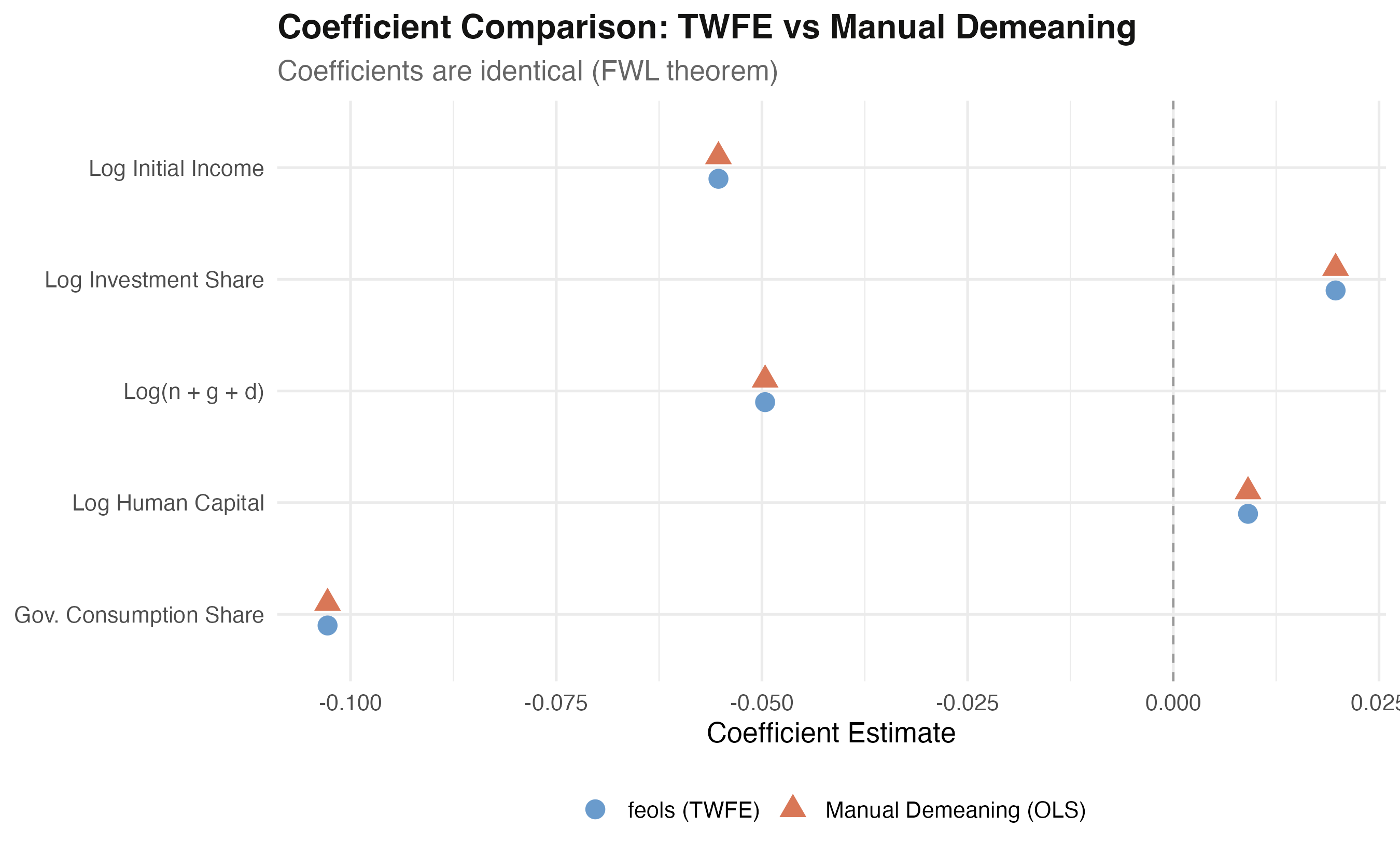
feols TWFE (blue circles) and manual-demeaning OLS (orange triangles) land on the exact same five positions.

This is the spoiler. Don’t explain every dot yet — just plant the surprise: feols with two-way fixed effects and base-R lm() on demeaned columns sit on top of each other for all five regressors. We earn this in Act II by deriving the demeaning formula, then come back to this picture as the payoff.

Where we’re going

• The lab: a balanced Barro panel — 150 countries × 8 periods
• The within transformation — subtract two means, add one back
• Frisch–Waugh–Lovell: why that must reproduce TWFE
• The catch: identical coefficients, wrong standard errors

Built straight from the post’s five learning objectives. Teaching deck, so an agenda earns its slide here.

The Investigation

Act II

The lab: 150 countries, 8 periods, every cell filled

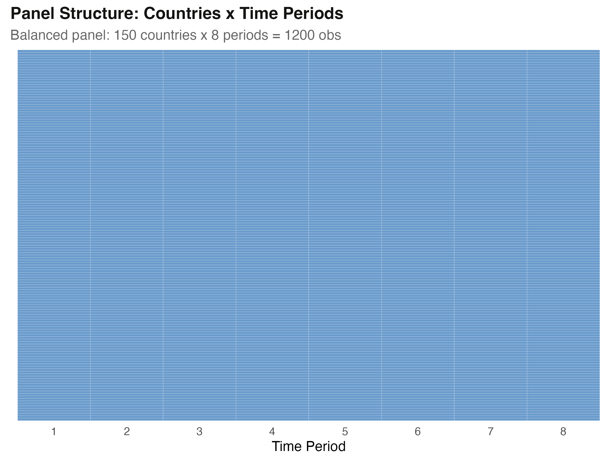
Every one of 150 countries appears in all 8 periods — a perfectly balanced 1,200-row panel.

A balanced panel is the ideal teaching setting: it lets us use the closed-form two-way demeaning (subtract country mean, subtract time mean, add grand mean) instead of the iterative projection unbalanced panels would require. The outcome is GDP-per-capita growth; the convergence regressor is log initial income, with four more controls.

TWFE is OLS with a country intercept and a period intercept

\[y_{it} = \alpha_i + \lambda_t + \beta x_{it} + u_{it}\]

Each country \(i\) gets its own intercept \(\alpha_i\); each period \(t\) gets its own \(\lambda_t\). Together they absorb every time-invariant country trait and every country-invariant shock.

Those intercepts are the “controls.” FWL says we can project them out instead of estimating them.

α_i soaks up persistent country differences (geography, institutions, long-run level); λ_t soaks up common shocks (a global recession, a productivity boom). This is exactly the “controls Z” that FWL lets us residualize away rather than carry in one giant dummy regression.

The within transformation: subtract two means, add one back

\[\tilde{x}_{it} = x_{it} - \bar{x}_{i\cdot} - \bar{x}_{\cdot t} + \bar{x}_{\cdot\cdot}\]

• \(\bar{x}_{i\cdot}\) — the country mean (removes persistent country level)
• \(\bar{x}_{\cdot t}\) — the time mean (removes the common period shock)
• \(+\,\bar{x}_{\cdot\cdot}\) — the grand mean, added back to undo double-subtraction

The double-dot accent here is the within-transformed variable. Demeaning growth for Brazil in 1965 means: subtract Brazil’s 8-period average, subtract 1965’s 150-country average, then add back the grand mean over all 1,200 rows. Repeat for every variable.

Why add the grand mean back? Miss it and you subtract the overlap twice

Subtract both the country mean and the time mean, and you remove the grand mean twice — it hides inside each. Add \(\bar{x}_{\cdot\cdot}\) back once to undo that.

Like a Venn diagram: remove both circles entirely and the overlap is deleted twice. Add the overlap back once.

Without the +grand-mean term, the demeaned variables are not centred at zero, the intercept is no longer ~0, and the FWL equivalence with TWFE breaks. The grand-mean correction is algebraically necessary, not cosmetic. This is also Exercise 1 in the post.

Frisch–Waugh–Lovell: residualize-then-regress equals the full regression

\[\hat{\beta}_{\text{TWFE}} = \hat{\beta}_{\text{OLS on demeaned data}}\]

The slope on \(x\) controlling for the dummies equals the slope from OLS on the residualized \(y\) and \(x\). TWFE is the special case where the controls are the country and time dummies.

Noise-cancelling headphones: subtract the engine hum from the signal first, then listen — same music as a silent room.

FWL is the theoretical guarantee behind the whole tutorial. “Either include all the dummies in one big regression, or project them out of both y and x and regress the residuals” — the coefficient on x is identical either way. Not approximately: exactly, as an algebraic identity.

Two routes to the slope — climb roped-up, or strip the ropes first

Route A — feols()

• growth ~ ... | id + time
• absorbs 150 country + 8 time FE
• iterative demeaning under the hood
• honest, FE-aware standard errors

Route B — hand-demean + lm()

• apply \(\tilde{x}_{it}\) to every column
• plain OLS, no FE machinery
• same point estimates (FWL)
• naive SEs — too small

The contrast is inseparable, so it earns one slide. Same summit, two paths. Route A is what everyone runs; Route B is the manual proof. They agree on β and disagree on the SE — the punchline of Act III.

Six lines reproduce TWFE by hand

VARS <- c("growth","ln_y_initial","log_s_k","log_n_gd","log_hcap","gov_cons")
cmean <- aggregate(panel[VARS], list(panel$id),   mean)   # country means
tmean <- aggregate(panel[VARS], list(panel$time), mean)   # time means
gmean <- colMeans(panel[VARS])                            # grand means

for (v in VARS)                                           # demean each column
  panel[[paste0(v,"_dm")]] <-
    panel[[v]] -
    cmean_lookup[[v]] -
    tmean_lookup[[v]] +
    gmean[v]

manual <- lm(growth_dm ~ ln_y_initial_dm + log_s_k_dm + log_n_gd_dm + log_hcap_dm + gov_cons_dm, panel)

Illustrative skeleton — the post uses dplyr group_by/left_join, but the algebra is exactly this: three means, the +grand-mean correction, then base-R lm() on the demeaned columns. We use lm() deliberately, not feols(), to prove no fixed-effects machinery is involved.

The demeaned columns are centred at zero — to 15 decimal places

Variable	Mean of demeaned column
growth_dm	−8.1e−17
ln_y_initial_dm	8.3e−15
gov_cons_dm	1.8e−16

All six means sit at \(10^{-15}\) or smaller — effectively zero. The transformation is implemented correctly.

This is the sanity check before the big claim. If the grand-mean term had been dropped, these means would not be zero and the intercept of the OLS step would not vanish. What’s left is pure within-variation — deviation from each country’s own average and each period’s common trend.

The Resolution

Act III

The two routes agree to 12 significant digits — max gap is machine epsilon

Variable	feols TWFE	manual OLS	difference
ln_y_initial	−0.055286	−0.055286	−4.2e−17
log_s_k	0.019725	0.019725	3.5e−18
gov_cons	−0.102795	−0.102795	−3.1e−16

all.equal() returns TRUE. Largest difference 3.05e−16 ≈ IEEE-754 machine epsilon (2.2e−16).

This is the central result. All five slopes are identical to at least 12 significant digits; the biggest discrepancy is floating-point noise, not estimation error. It is an exact algebraic identity guaranteed by FWL, verified empirically on real-ish data.

One number, two methods, zero disagreement

−0.055286

Convergence \(\hat\beta\) on log initial income — identical from feols() and from lm() on demeaned data

A country one log-point poorer at the start of a period grows about 5.5 percentage points faster, conditional on country and period fixed effects — strong conditional β-convergence (t = −14.77). The headline is not the economics but the equivalence: the same number falls out of two notations of the same calculation.

Demeaning is the picture: wide spread collapses to within-variation

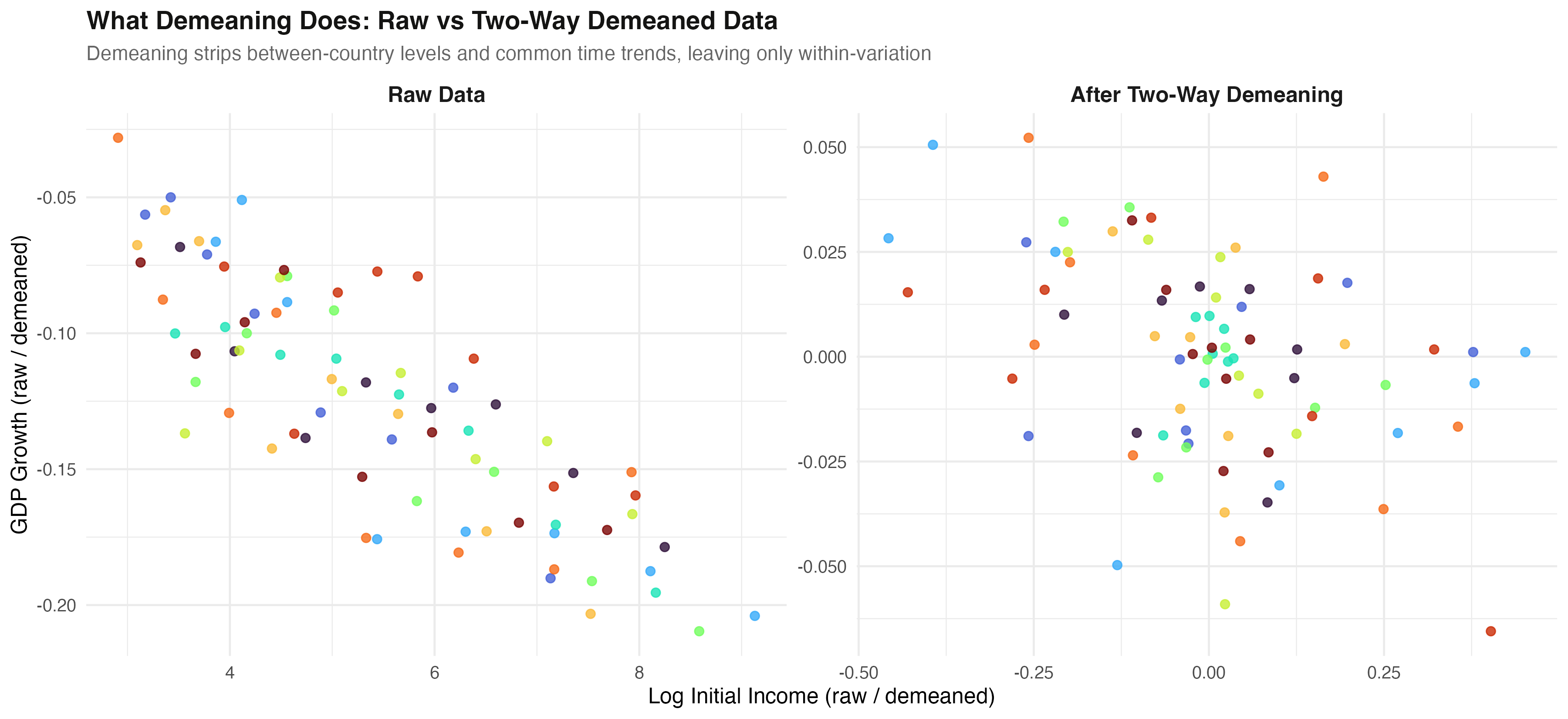
Raw cross-country spread on the left (x from ~3 to 9); after two-way demeaning, the same data compresses to roughly −0.5 to 0.3 around zero.

This is what TWFE throws away and what it keeps. The between-country income differences and common time trends are stripped out, leaving only within-variation — the deviations that actually identify β. Any variable with no within-variation (geography, colonial origin) becomes zero everywhere and drops out. That is why FE cannot estimate time-invariant characteristics.

Inside one country: observed minus two means, plus the grand mean

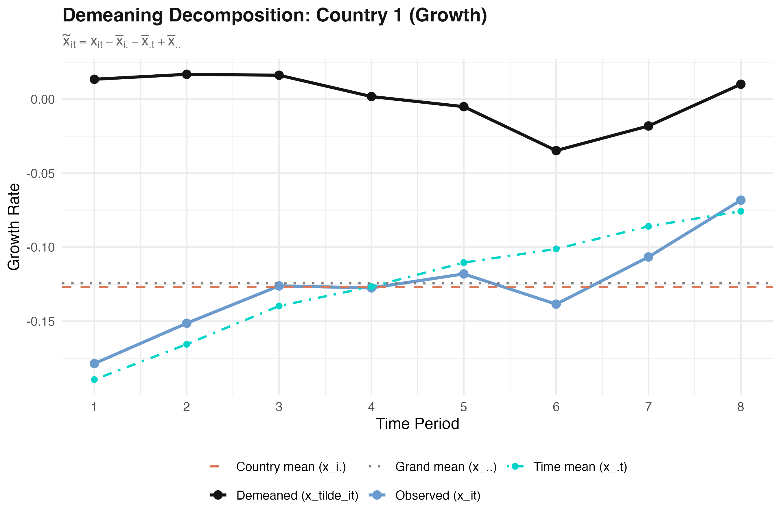
Country 1: observed growth (blue), country mean (orange dashed), time means (teal), grand mean (gray), and the demeaned residual (black) fluctuating around zero.

The formula made concrete for one country across all 8 periods. Observed growth declines from about −0.18 to −0.07; the flat orange line is the country mean (−0.127); the teal line is the time means (the common trend); the gray dotted line is the grand mean (−0.124). Subtract the first two, add the last, and you get the black residual — the within-country, within-period deviation TWFE uses.

The catch: identical coefficients, but lm() standard errors are too small

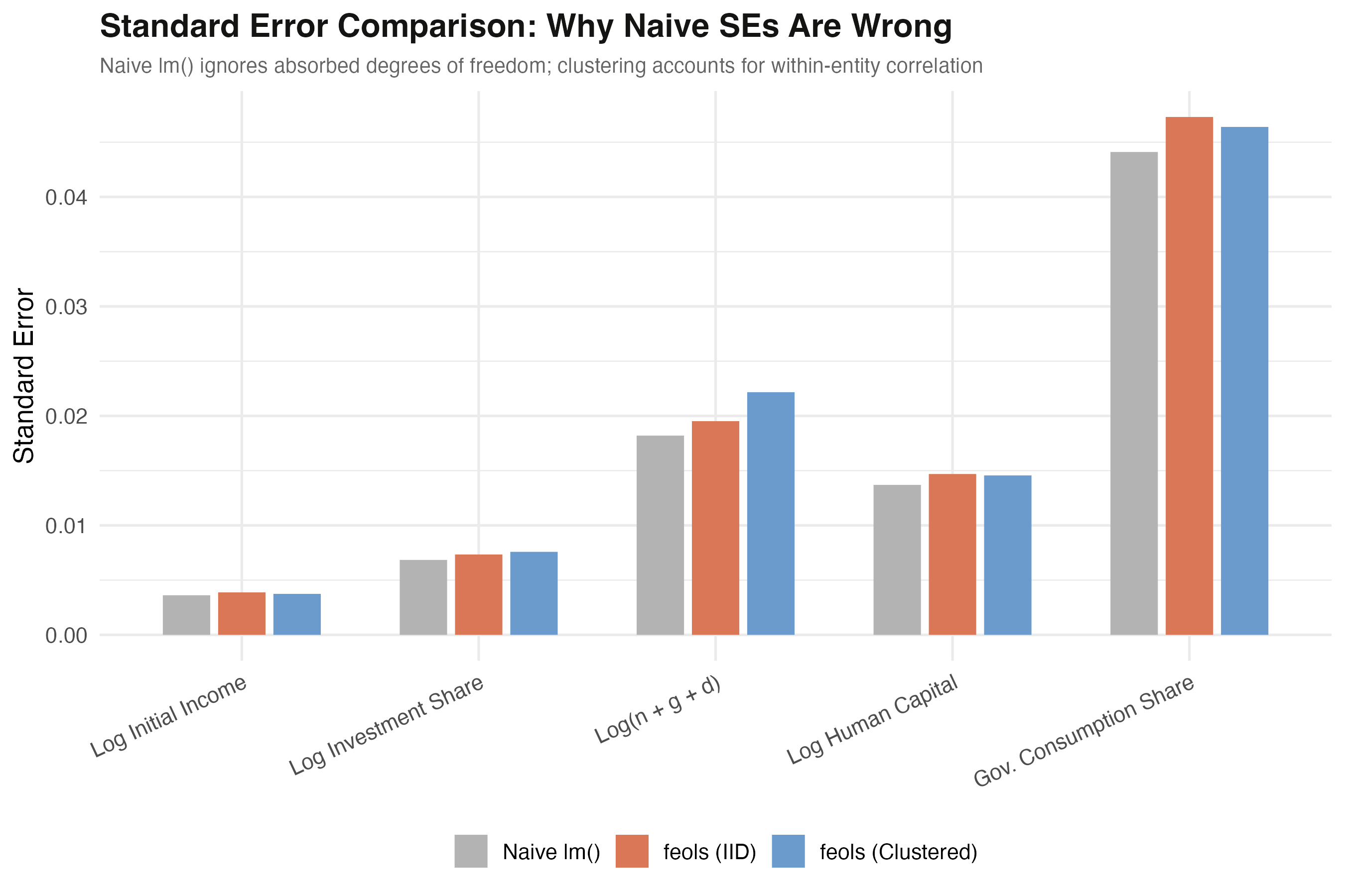
For every regressor the naive lm() bar (gray) is shorter than feols IID (orange) and clustered (blue).

The point estimates are exact, but inference is not free. lm() doesn’t know that 157 degrees of freedom were spent estimating 150 country + 8 time effects (minus 1). It divides by df = 1,195 instead of the correct 1,038, so its SEs run 7–22% too small. The biggest gap is log(n+g+d): 0.0182 naive vs 0.0222 clustered.

The strongest objection — and the answer

Objection. “If lm() on demeaned data nails the coefficients, why not just use it and skip fixest?”

Response. Because correct points \(\neq\) correct inference. lm() understates SEs by 7–22% — narrow CIs, inflated \(t\)-stats. feols() fixes the df and clusters for serial correlation. Use a panel estimator for any test.

Steelman, don’t strawman. The manual route is a teaching device and a proof — it is genuinely the same calculation for β. But shipping it in applied work would publish over-confident standard errors. The convenience of lm() is exactly the trap.

What demeaning teaches: FE identifies within variation, nothing else

• Time-invariant regressors have country mean = themselves → demean to zero → dropped
• The grand-mean correction is not optional — omit it and FWL breaks
• Within R² = 0.177 vs adjusted R² = 0.755: the FE absorb most of the variance

The three practical insights from the Discussion section, compressed. The within/total R² gap is the quantitative face of “fixed effects do most of the absorbing.” This is also why you can’t recover the effect of geography from a country-FE model: there’s no within-country variation left to use.

TWFE is just OLS on two-way-demeaned data — agree on β, never trust its naive SE.

The single sentence to remember — the resolution of the Act-I hook. Open the box and TWFE is ordinary least squares on data with the country and time means swept out; the coefficient is exact, the standard error is not.