Difference-in-Differences for Policy Evaluation

Does the minimum wage cut teen jobs? A modern DiD walkthrough in R

−0.057true overall ATT · TWFE missed by ⅓

−0.065doubly robust · stable everywhere

0.67HonestDiD breakdown · robust

Carlos Mendez

Nagoya University (GSID)

June 11, 2026

The Tension

Act I

Same panel, same question — but the answer depends on the estimator you trust

Did raising the minimum wage cost teens their jobs? Run the textbook two-way fixed-effects (TWFE) regression and you get \(-0.038\).

Run the modern estimator on the same counties and you get \(-0.057\) — half again as large. Which one is right?

This is the hook. The same data give two different answers. The whole talk is about why the textbook number is wrong, by how much, and what to use instead. The estimand throughout is the ATT — the average effect on counties that actually raised their minimum wage, not the population at large.

A frozen federal floor of $5.15 turned the states into a natural experiment

From 2001–2007 the federal minimum wage sat frozen at $5.15/hour, while states raised their own floors at different times.

Counties fall into cohorts indexed by their first-increase year \(G \in \{0, 2004, 2006\}\): 102 treated in 2004, 226 in 2006, and 1,417 never-treated.

Staggered adoption: there is no single “before” and “after” for the country — each state has its own clock.

Staggered treatment timing is the source of all the trouble. With a single common treatment date, TWFE is fine. The moment treatment dates differ across units, TWFE starts making comparisons it should not. 8,725 county-year observations, 1,745 counties, 2003–2007.

TWFE understates the true effect by a third — that gap is the whole talk

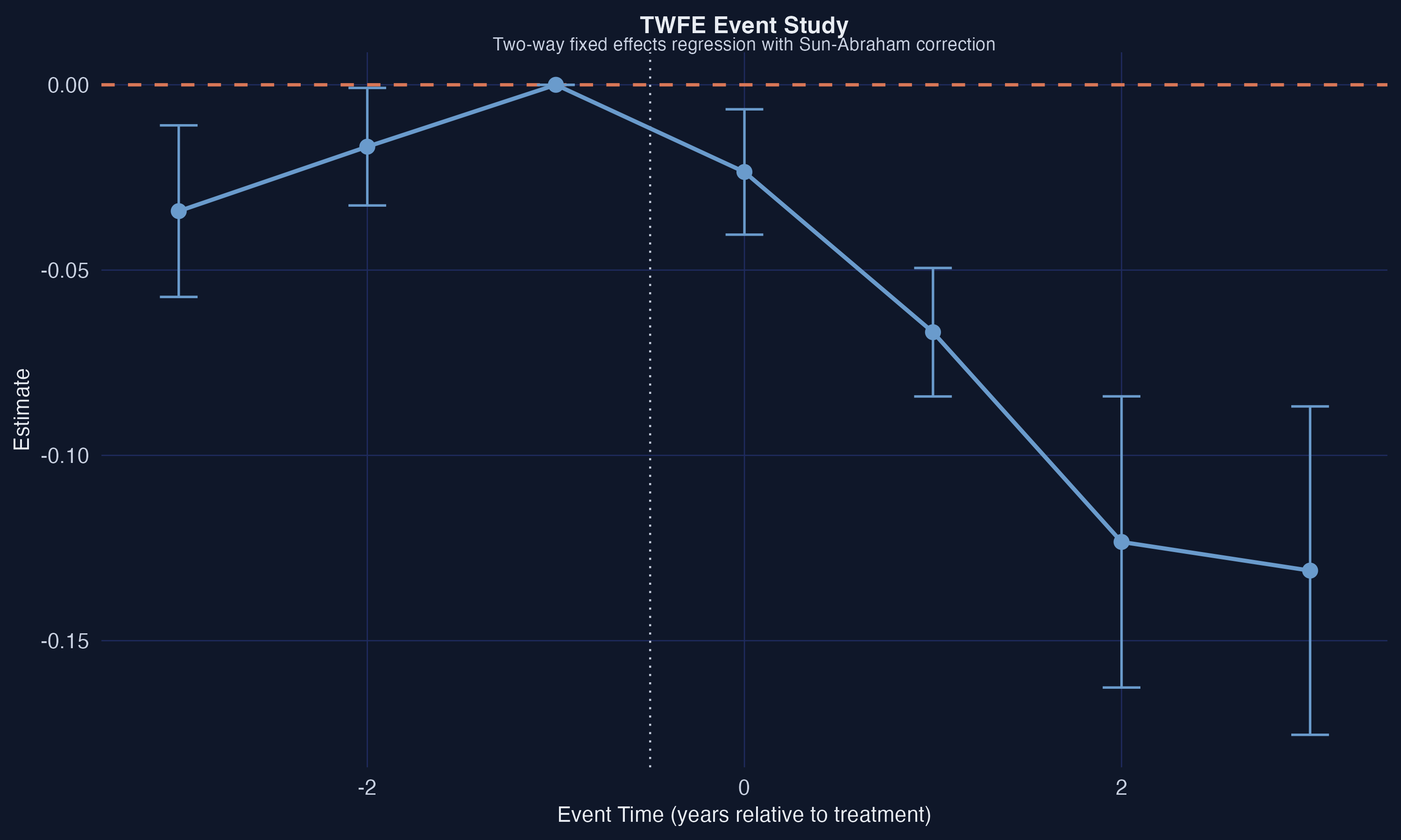
TWFE event study (Sun-Abraham interaction-weighted estimator). A pre-trend wobble at event time \(-3\); effects deepen after treatment.

Spoiler slide. Don’t dwell on every coefficient — just plant the idea that even the “corrected” TWFE event study shows a pre-trend at e=−3 and growing post-treatment effects. We will earn the cleaner Callaway–Sant’Anna picture in Act II and come back to it.

Where we’re going

• The lab: a staggered minimum-wage panel with a never-treated control
• Why TWFE breaks — forbidden comparisons and negative weights
• Callaway–Sant’Anna group-time \(\mathrm{ATT}(g,t)\), then aggregate
• Doubly robust covariates, then stress-test parallel trends with HonestDiD

The Investigation

Act II

Identification rests on one assumption: parallel trends

\[\mathrm{ATT} = E[\Delta Y_{t^{\ast}} \mid D=1] - E[\Delta Y_{t^{\ast}} \mid D=0]\]

The treated group’s change in outcomes, minus the comparison group’s change. Valid only if both groups would have moved in parallel absent treatment.

The estimand is the ATT — the effect on the counties that actually raised their wage.

Notation: D=1 treated, D=0 untreated, ΔY the pre-to-post change. Parallel trends is the identifying assumption, and it is not directly testable — pre-trends near zero are necessary but not sufficient. State this estimand clearly: ATT, not ATE. We never claim an effect for counties that didn’t change their wage.

TWFE silently uses already-treated counties as controls — a forbidden comparison

With staggered timing, TWFE mixes two kinds of comparison:

• Good: treated vs not-yet-treated or never-treated
• Bad: later-treated vs already-treated — the control is itself under treatment

Like grading a student’s improvement against classmates who already took the test — the “control” already saw the answer key.

Under treatment-effect heterogeneity the TWFE coefficient is a weighted average of group-time effects, and some weights go negative. In principle TWFE could return a negative estimate even if every true effect were positive. This is the de Chaisemartin–D’Haultfœuille / Goodman-Bacon critique in one slide.

The fix: estimate one clean effect per cohort × period, then aggregate

\[\mathrm{ATT}(g,t) = E[\,Y_t(g) - Y_t(0) \mid G = g\,]\]

The effect for cohort \(g\), measured in calendar period \(t\) — each cell compared only to clean (never- or not-yet-treated) controls.

Callaway–Sant’Anna (2021): separate identification from estimation. Build the grid of \(\mathrm{ATT}(g,t)\) first, average it later.

This is the conceptual heart. Instead of one regression coefficient, we get a grid of building-block parameters, each identified by a clean comparison under parallel trends. No forbidden comparisons can enter, by construction.

Six lines of did replace the broken regression

attgt <- did::att_gt(yname = "lemp",            # log teen employment
                     idname = "id", gname = "G", # unit id, first-treatment cohort
                     tname = "year",
                     control_group = "nevertreated",
                     base_period = "universal",
                     data = data2)
attO  <- did::aggte(attgt, type = "group")       # overall ATT
attes <- did::aggte(attgt, type = "dynamic")     # event study

att_gt() estimates every ATT(g,t). aggte() rolls them up two ways: a group/cohort overall ATT, and a dynamic (event-time) aggregation. control_group = “nevertreated” picks the 1,417 clean controls; base_period = “universal” compares everything to t = g−1.

Each cohort’s effect deepens with exposure — dynamics TWFE flattens away

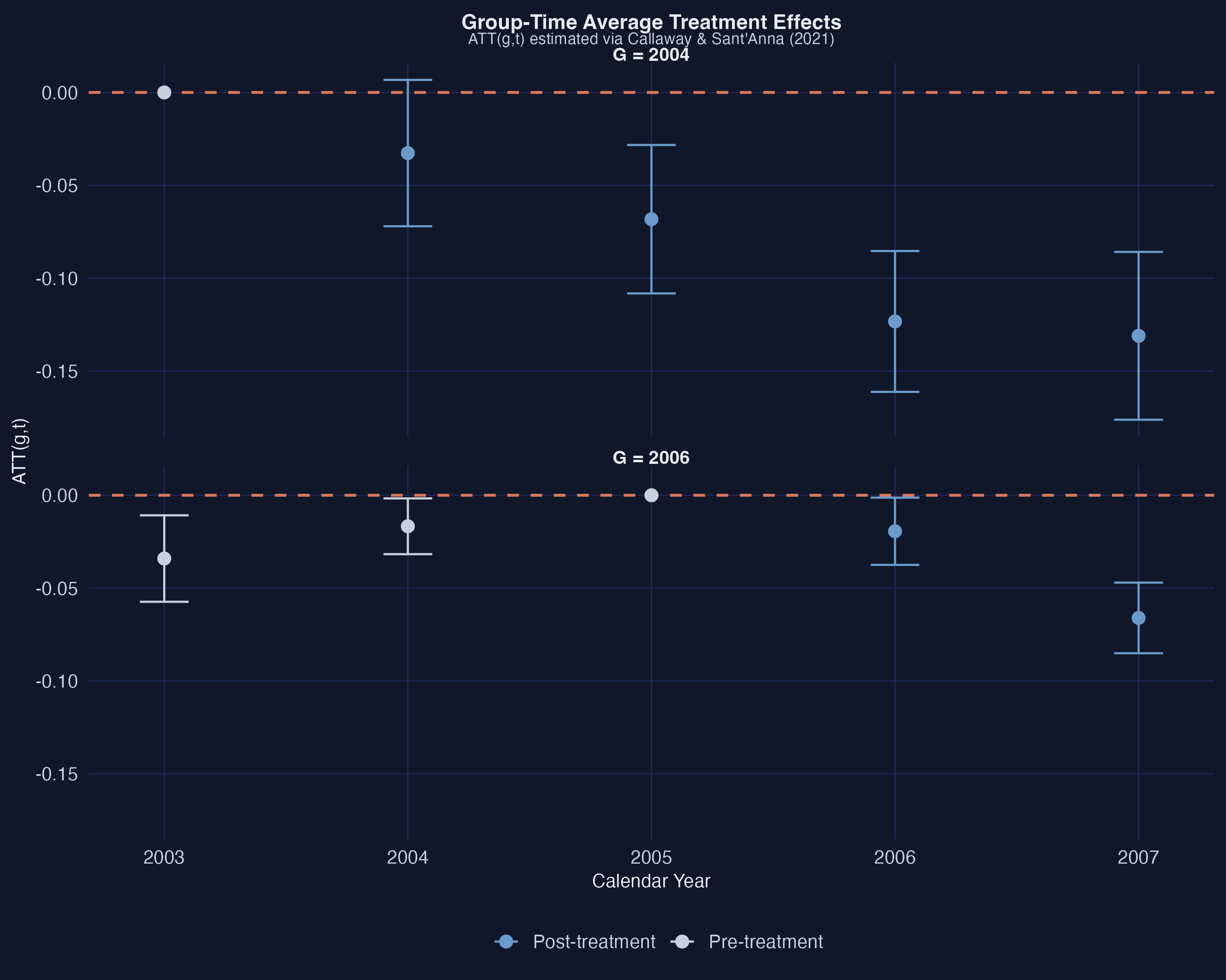
Group-time ATTs by cohort (Callaway–Sant’Anna). The G=2004 line falls further every year of exposure.

For G=2004: −0.033 on impact, −0.068 after a year, −0.123 after two, −0.131 after three. For G=2006: −0.019 on impact, growing to −0.066. The G=2006 pre-period value of −0.034 at e=−3 is the warning flag we revisit in HonestDiD.

Aggregated cleanly, the true overall ATT is −0.057 — not TWFE’s −0.038

Estimator	Overall ATT	SE	Sig. 5%?
TWFE	−0.038	0.008	yes
Callaway–Sant’Anna	−0.057	0.008	yes

TWFE understated the negative effect by about a third — attenuated toward zero.

The overall ATT weights each ATT(g,t) by group size and number of post periods. Group-level: G=2004 at −0.089 (treated longer, more dynamics) vs G=2006 at −0.043. The headline contrast is −0.057 vs −0.038.

The trajectory is clear: small on impact, large after three years

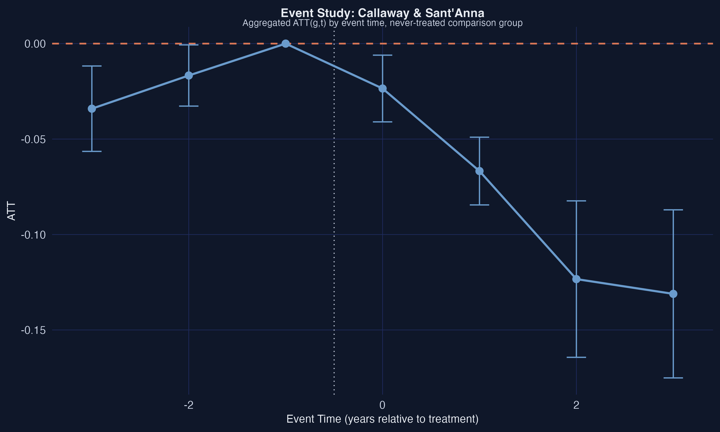
Event-study aggregation. Pre-trends hover near zero (with a wobble at \(e=-3\)); post-treatment effects grow monotonically.

e=0: −0.024; e=1: −0.067; e=2: −0.123; e=3: −0.131. All post-treatment effects significant. The pre-trend at e=−3 (−0.034) is marginally significant — flag for HonestDiD. e=−2 (−0.017) is not significant.

Where does TWFE’s bias come from? 64% pre-trend contamination, 36% bad weights

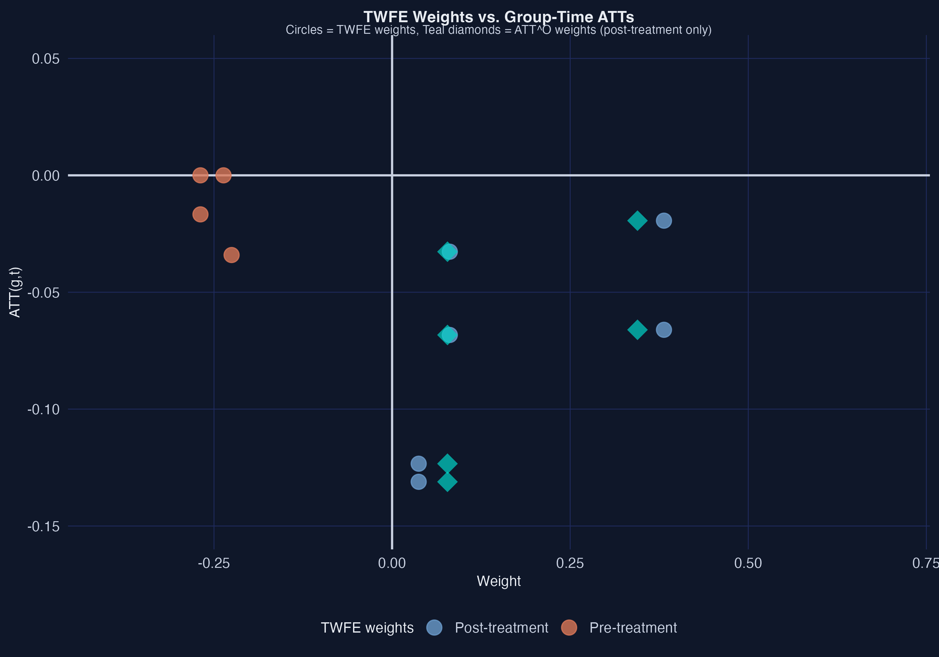
TWFE weight scatter. Orange pre-treatment cells get nonzero TWFE weight (they should get zero); blue post-treatment weights differ from the proper teal \(\mathrm{ATT}^O\) weights.

twfeweights decomposition: both TWFE and ATT^O are weighted averages of the SAME ATT(g,t) — only the weights differ. Total bias 0.019. 64.2% is pre-treatment contamination (TWFE puts weight on pre-periods that should be exactly zero); 35.8% is improper post-treatment weighting.

Conditioning on covariates barely moves the answer: −0.065, three ways

Method	Overall ATT	SE
Unconditional	−0.057	0.008
Regression adj.	−0.064	0.008
IPW	−0.065	0.008
Doubly robust	−0.065	0.008

Three independent modeling routes agree — no model-dependence artifact.

Conditional parallel trends: trends need only be parallel after conditioning on log population and log average pay. Doubly robust = belt and suspenders: consistent if EITHER the outcome regression OR the propensity score is right. Going from −0.057 to −0.065 is a small, sensible move once county characteristics are netted out.

Covariates also clean up the pre-trend — the early wobble shrinks and loses significance

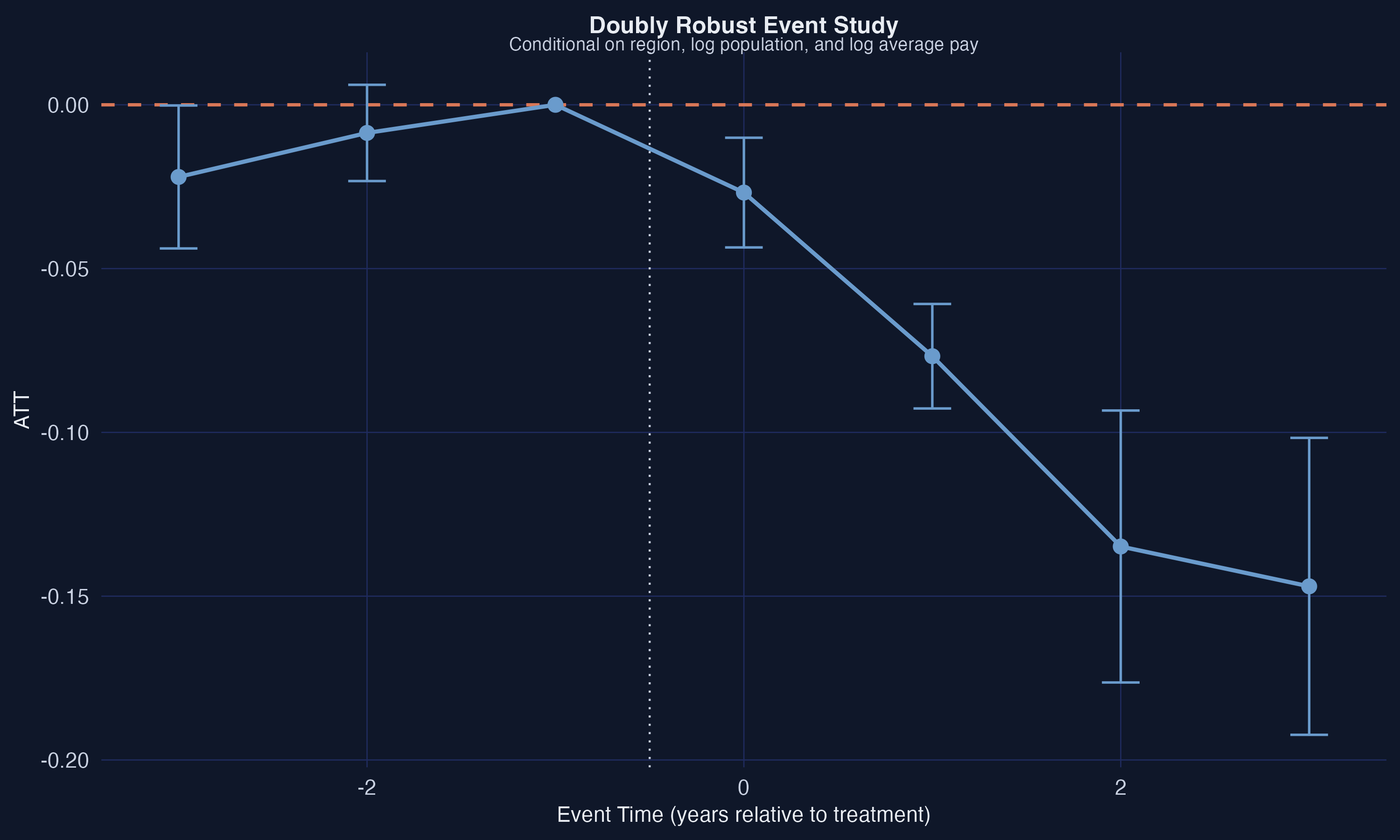
Doubly robust event study (controlling for log population and log average pay). The \(e=-3\) pre-trend shrinks from \(-0.034\) to \(-0.022\) and is no longer significant.

Post-treatment under DR: −0.027 (e=0), −0.077 (e=1), −0.135 (e=2), −0.147 (e=3). The improved pre-trend suggests the unconditional wobble was partly differences in county characteristics between treated and control groups, not a true violation.

−0.065 survives every researcher choice we throw at it

−0.065

doubly robust ATT · identical under varying base period (−0.065), not-yet-treated controls (−0.065); anticipation pulls it to −0.040

Robustness battery: varying base period −0.0646, not-yet-treated comparison −0.0649, both essentially identical to the −0.065 baseline. Allowing one period of anticipation drops it to −0.040 — sensible, since part of the effect then lands in the pre-period and is excluded from “post.”

The Resolution

Act III

How fragile is this? The on-impact effect breaks only at \(\bar M \approx 0.67\)

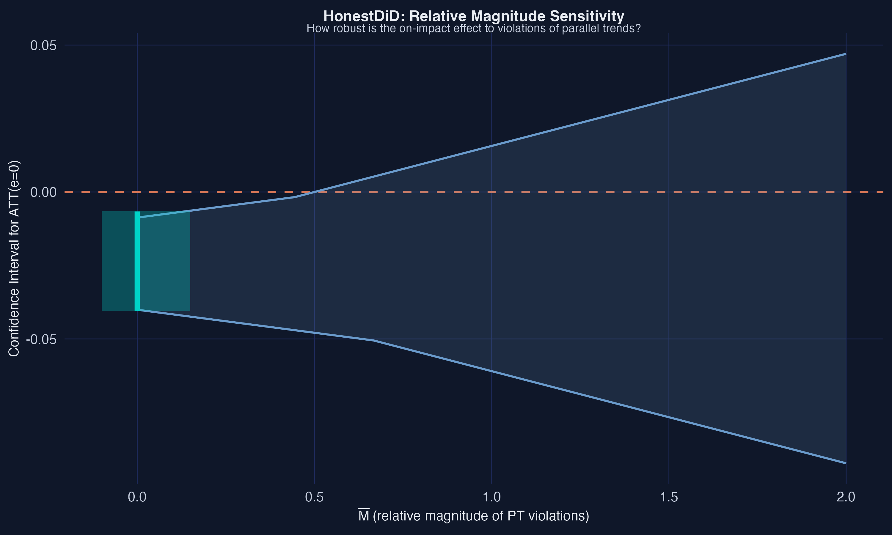
HonestDiD sensitivity: the on-impact CI widens as allowed parallel-trends violations grow. It first touches zero near \(\bar M = 0.67\).

HonestDiD (Rambachan–Roth 2023, relative-magnitude variant): how big can a post-treatment parallel-trends violation be, relative to the worst pre-treatment deviation, before the result breaks? Original CI [−0.040, −0.007]. As Mbar rises the band widens; near Mbar≈0.67 it first includes zero. So the effect tolerates violations up to ~67% of the observed pre-trend — robust to moderate, not large, violations.

A dose-response emerges: each extra $1 cuts teen jobs ~5% at one year, ~9% at three

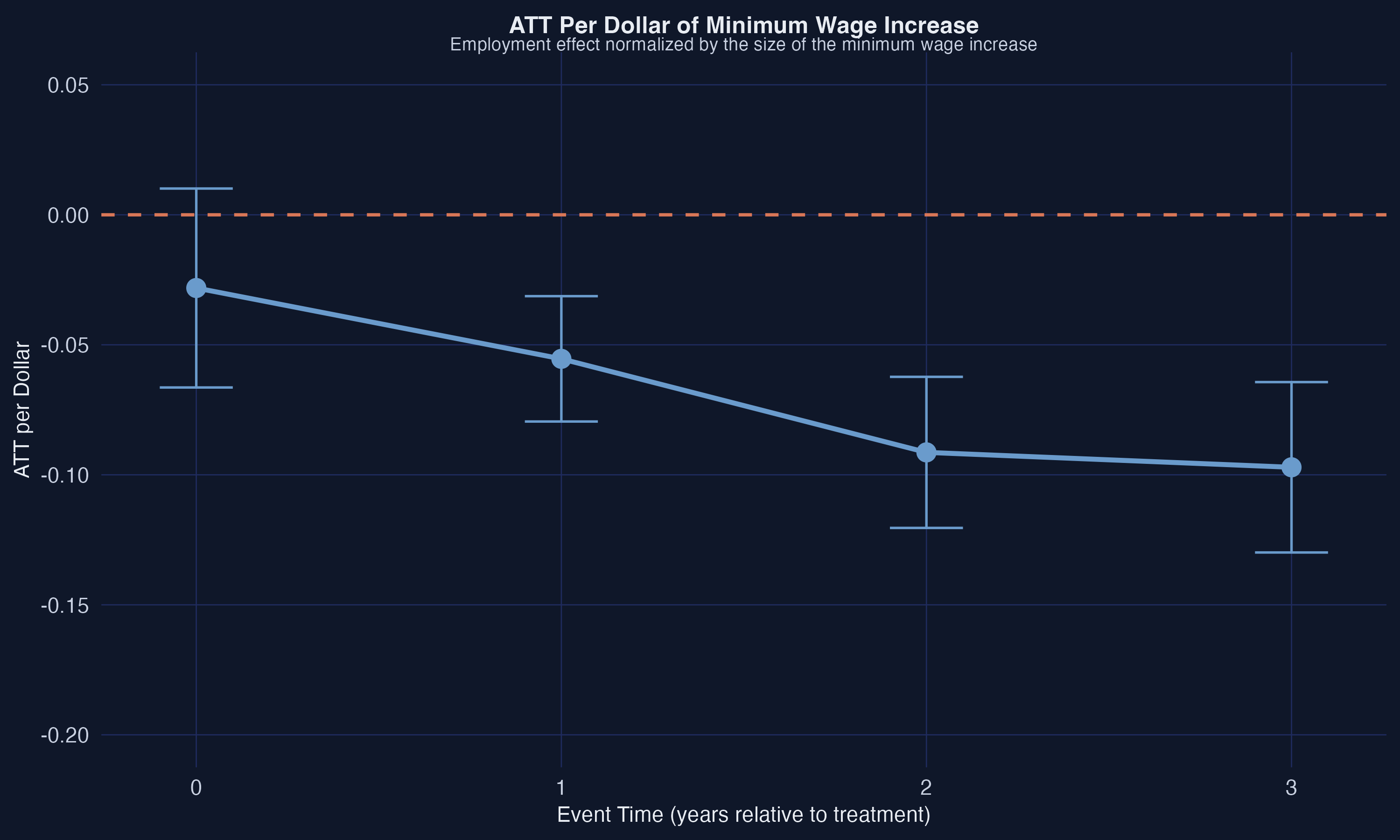
ATT per dollar of minimum-wage increase. The per-dollar effect deepens with cumulative exposure.

Normalizing by the actual size of each state’s increase: −0.028 on impact (not quite significant), −0.055 (e=1), −0.091 (e=2), −0.097 (e=3). A $1 rise ≈ a 5.3% employment drop after one year, 9.2% after three. The state minimum-wage trajectories (figure r_did_07) show how heterogeneous the doses are — Illinois early and large, Florida and Colorado smaller and later.

Does machine-disciplined DiD make this causal? Not by itself

Objection. Fancy estimators and covariate adjustment can’t manufacture identification — maybe minimum-wage states were just on a different employment path.

Response. Correct, and we never claim otherwise. The ATT is identified only under (conditional) parallel trends. HonestDiD makes the dependence on that assumption explicit and quantifies exactly how much violation the conclusion can absorb.

Steelman, don’t strawman. Callaway (2022) explicitly frames this as a methodological illustration, not a settlement of the minimum-wage debate. The pre-trend at e=−3 and the Mbar≈0.67 breakdown are honest about the limits. Convergence with the lagged-outcomes strategy (ATT −0.061) adds confidence but does not replace the assumption.

What to take home: clean comparisons change the number and the story

• TWFE understated the ATT by ~⅓ (−0.038 vs −0.057); 64% of the bias is pre-trend contamination
• The doubly robust ATT of −0.065 is stable across methods, controls, and base periods
• Effects accumulate: −0.027 on impact to −0.147 after three years; ~5% per $1 at one year, ~9% at three
• Robust to parallel-trends violations up to \(\bar M \approx 0.67\) — suggestive, not bulletproof

The four numbers a student should walk out with. The meta-lesson: DiD is an identification strategy, not a regression. The estimator you pick, the comparison group, and the credibility of parallel trends all change the answer.

Let the design, not the regression default, choose your comparisons.

The single takeaway, resolving the Act-I hook. Under staggered adoption and heterogeneous effects, the textbook TWFE coefficient is a contaminated weighted average. Estimate clean group-time effects, aggregate deliberately, and stress-test parallel trends — the difference between −0.038 and an honest −0.057.