DiD with Geocoded Microdata

When distance defines treatment: the ring design

−5.78%parametric ring DiD at 0.1 mi

−20.6%nonparametric, closest 300 feet

52%spread from ring-choice alone

Carlos Mendez

Nagoya University (GSID)

June 11, 2026

The Tension

Act I

When the treatment is a point in space, the radius you choose dictates the answer

A registered sex offender moves into a neighborhood. To measure the price effect, compare homes close to the address with homes a little farther — before and after arrival.

But “close” is a choice. Linden & Rockoff drew the line at 0.1 mile. Move it, and the answer moves with it. Which radius?

This is the central tension of spatial DiD: distance, not policy assignment, defines who is treated. The radius is not a nuisance parameter — it is part of the question being asked. Donohue-Levitt-style identification, but the running variable is meters from a point.

One number hides the story: −5.78% on average, but −20.6% within 300 feet

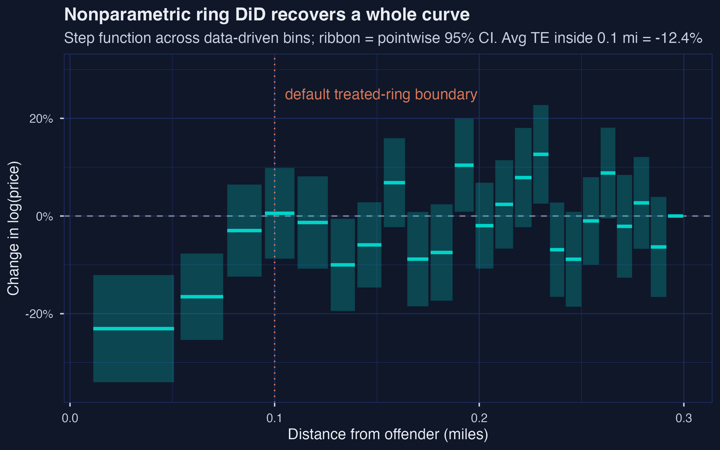
Nonparametric ring DiD on Linden-Rockoff: 23 bins; two closest bins at −20.6% and −15.2%; the curve crosses zero at \(d \approx 0.094\) mi.

Spoiler figure — don’t unpack every bin yet. Just plant the tension: the headline parametric average (−5.78%) and the closest-bin estimate (−20.6%) differ by a factor of two, and the effect dies out right around the cutoff the original authors guessed. We earn this picture in Act III.

Where we’re going

• The ring design: distance defines treated vs control
• A simulated world with a known answer to test the estimators
• The parametric ring DiD — and why its headline wobbles with the radius
• The nonparametric alternative — let the data trace the whole curve
• Linden & Rockoff: reconciling −5.78% with −20.6%

The Investigation

Act II

The estimand is an ATT — and the radius \(\bar d\) is baked into it

The ring DiD estimates the average treatment effect among the treated:

\[\tau = E[\Delta Y \mid d \le \bar d] - E[\Delta Y \mid d > \bar d]\]

Crucially, \(\bar d\) appears inside the expectation. Change the cutoff and you change the estimand — not just the precision.

State the estimand out loud: ATT inside the ring, with the outer ring as the counterfactual trend. The identifying assumption is local parallel trends (Butts 2023, Assumption 2). The cross-section admits no formal pre-trends test — the nonparametric curve’s behavior past the cutoff is the closest informal check we get.

Distance buys identification but spends sample: 6% treated, 28% control, 65% dropped

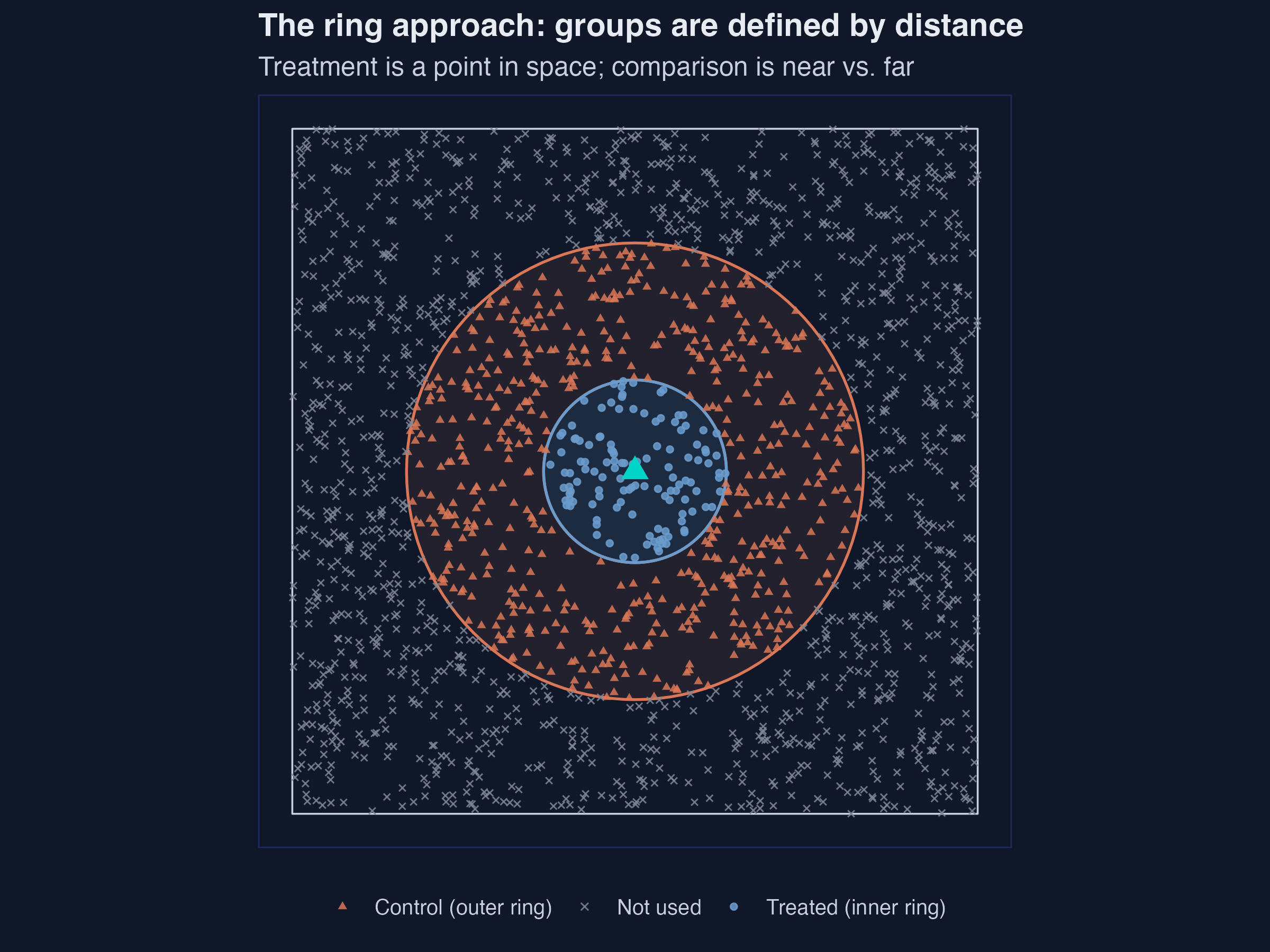
Toy ring geometry: 126 treated, 566 control, 1,308 dropped out of 2,000 random points.

Of 2,000 random homes, only 126 (6.3%) land in the treated disk, 566 (28.3%) in the control donut, and 1,308 (65.4%) are too far to enter. That 6/28/65 split is the price of the design: a small treated group anchors everything. On Linden-Rockoff the inner ring still holds ~1,100 sales, so it is feasible.

A ring DiD is a 2×2 DiD whose groups are defined by distance

The textbook two-way fixed-effects form, with \(\Delta Y\) first-differenced:

\[Y_{it} = \alpha_i + \gamma_t + \tau\, D_i P_t + \varepsilon_{it}\]

Estimator	Estimate	SE	True
First-differences	0.3097	0.0258	0.30
Two-way FE	0.3097	0.0258	0.30

The two are algebraically identical — that is why the ring DiD is one line of feols().

On a 500-unit panel with true effect 0.30, first-differences and TWFE return numerically identical estimates (0.3097) and SEs (0.0258), both within one SE of truth. The equivalence is exact, not approximate — it licenses writing the ring DiD as one regression on first-differenced outcomes.

Build a world where the truth is known: \(\tau(d)\) vanishes exactly at 0.75 mi

\[\tau(d) = 1.5 \cdot \exp(-2.3\, d) \cdot \mathbf{1}\{d \le 0.75\}\]

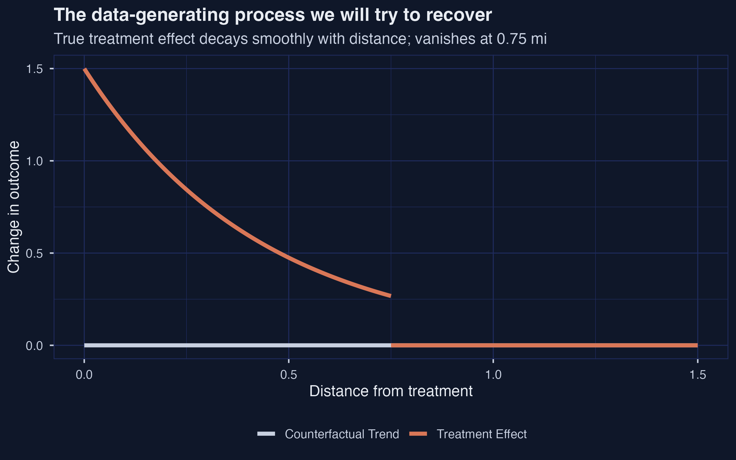
True treatment-effect curve: \(\approx 1.5\) at the point, decaying smoothly, zero past 0.75 mi; mean over the affected region \(= 0.726\).

10,000 units, distance uniform on [0, 1.5]. The effect is largest at the point (≈1.5), decays smoothly, and is exactly zero beyond 0.75 mi — what Butts calls d_t. The average true effect across [0, 0.75] integrates to 0.726. That number is the benchmark every estimator must recover.

With the correct radius, the parametric estimator nails the truth: 0.726

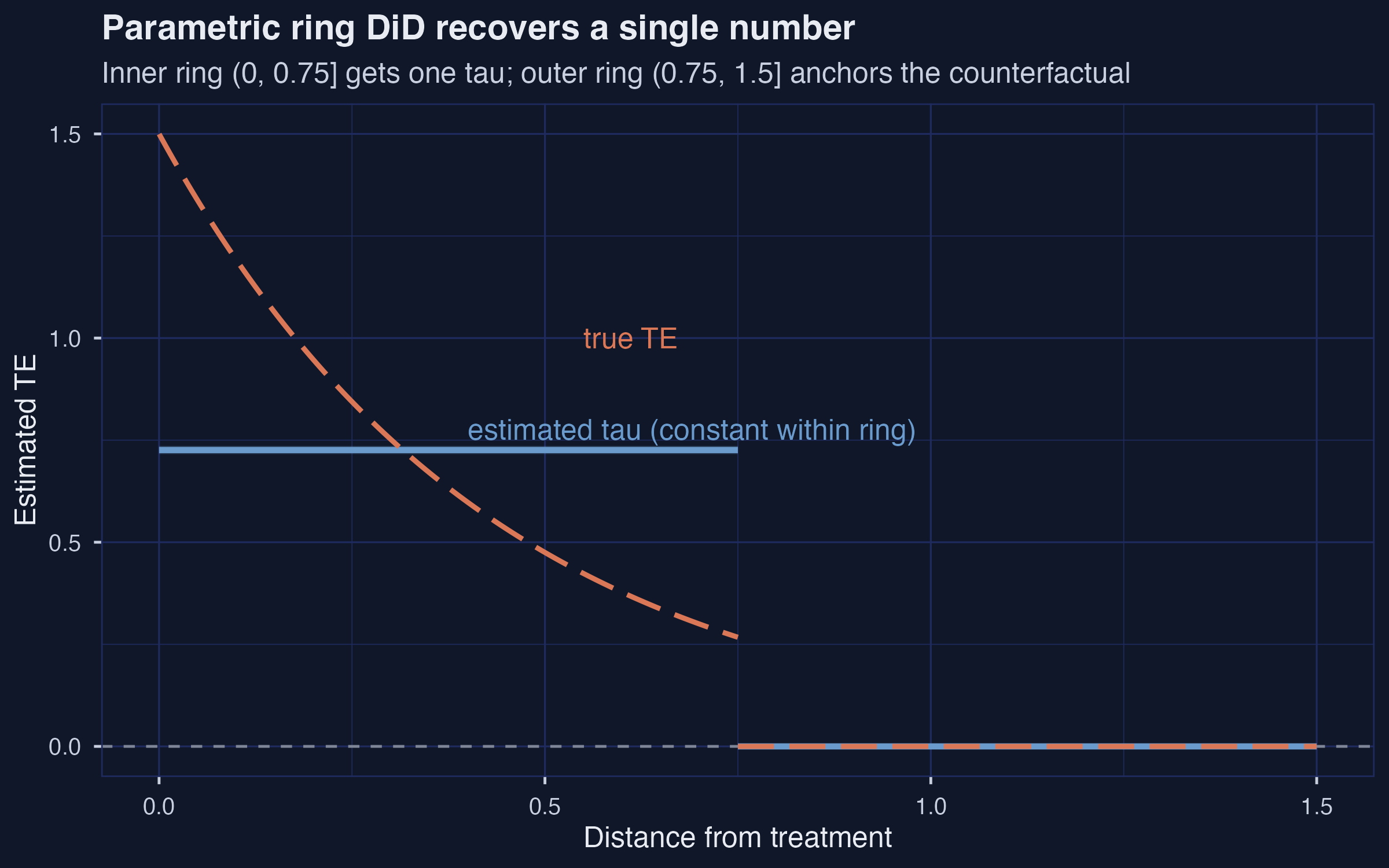
Parametric ring DiD at the correct cutoff recovers the truth: \(\hat\tau = 0.726\), 95% CI \([0.716, 0.736]\).

Set inner = (0, 0.75], outer = (0.75, 1.5] — the exact distance where effects vanish — and the estimator returns 0.726 with SE 0.005, CI centered on truth. The outer ring is normalized to zero by construction; it is the counterfactual trend. Strongest internal-validity check there is. The catch: we know 0.75 only because we wrote the DGP. In real data, d_t is the unknown.

Same data, three radii, three answers: 0.913 / 0.726 / 0.456

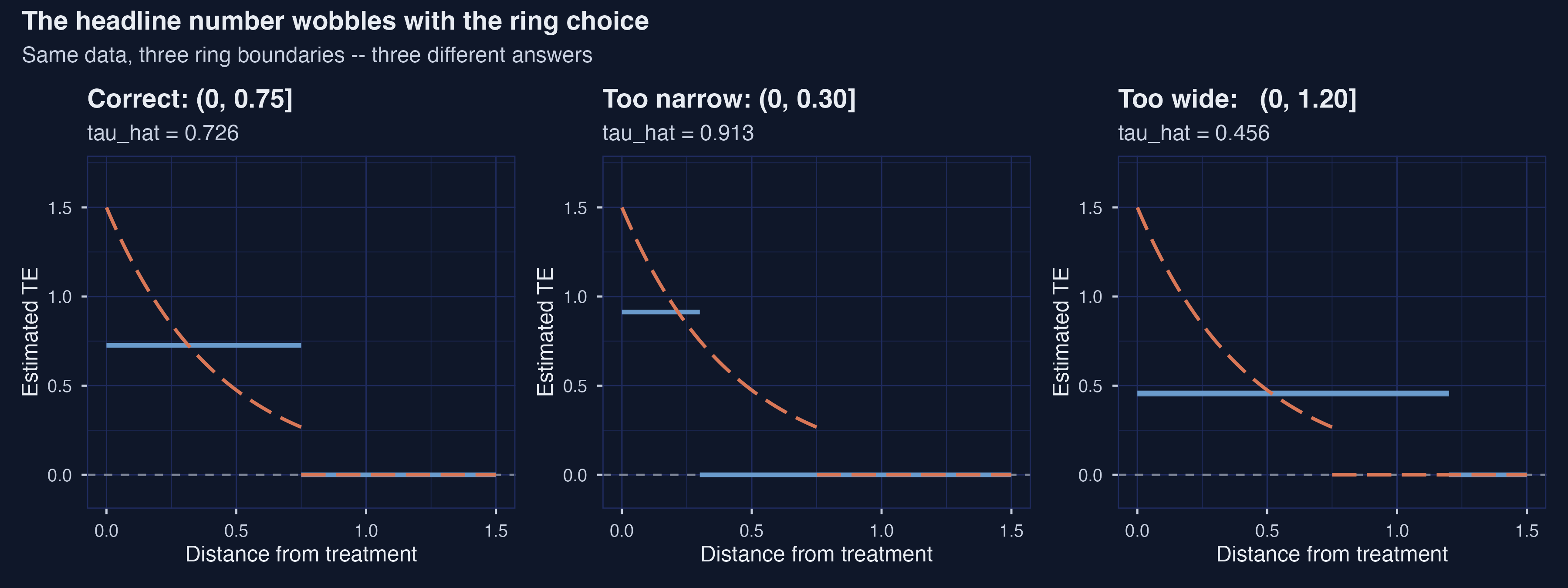
Same data, three ring choices: 0.913 (too narrow), 0.726 (correct), 0.456 (too wide). Both bad-case 95% CIs exclude the truth.

Choice	\(\hat\tau\)	Bias
Too narrow (0, 0.30]	0.913	+25.7% — averages the steepest slice
Correct (0, 0.75]	0.726	none
Too wide (0, 1.20]	0.456	−37.1% — dilutes with zero-effect units

Hold data, seed, and regression fixed; only the cutoff moves. Too-narrow over-states (+25.7%) by averaging only the steep part; too-wide attenuates (−37.1%) by absorbing unaffected units. Neither is noise — both bad-case CIs strictly exclude 0.726. Ring choice is part of the estimand, not a precision lever.

The parametric ring DiD is one line of feols() on first-differenced outcomes

ring_dgp <- ring_data |>
  mutate(treat_ring = as.integer(dist <= 0.75)) |>
  feols(delta_y ~ treat_ring, cluster = "neighborhood", data = _)

delta_y is the first-differenced outcome; treat_ring is the 0/1 inner-ring indicator. The whole estimator is that one regression.

Because of the 2×2 equivalence, the entire parametric ring estimator is a single feols() call on first-differenced log prices with a treated-ring dummy and neighborhood-clustered errors. The Linden-Rockoff sibling swaps in close_post_move and srn_year fixed effects — same shape.

Let the data choose: partition distance into bins and trace the whole curve

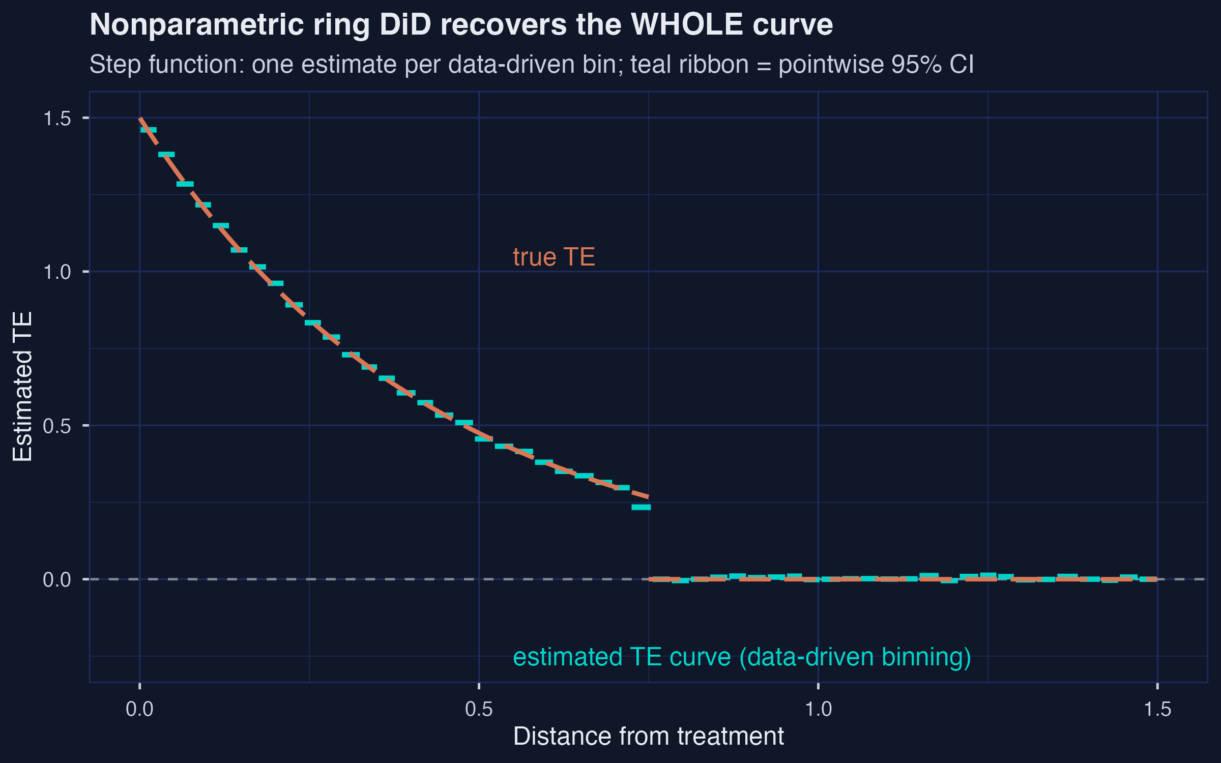
The nonparametric estimator recovers the whole TE curve — 53 quantile-spaced bins, no cutoff committed up front; left-most bin \(\hat\tau = 1.461\) vs truth 1.5.

Where the parametric estimator gives one number, binsreg gives a step function. Partition distance into L quantile-spaced bins (L chosen by an MSE criterion), fit a constant in each, difference from the last untreated bin. On the DGP it picks 53 bins; the left-most returns 1.461 (truth 1.5), steps down monotonically, crosses zero near 0.75 mi. No cutoff needed — the rebuttal to ring-choice fragility.

Eyeballing the cutoff is the same fragility in disguise — three bandwidths, three radii

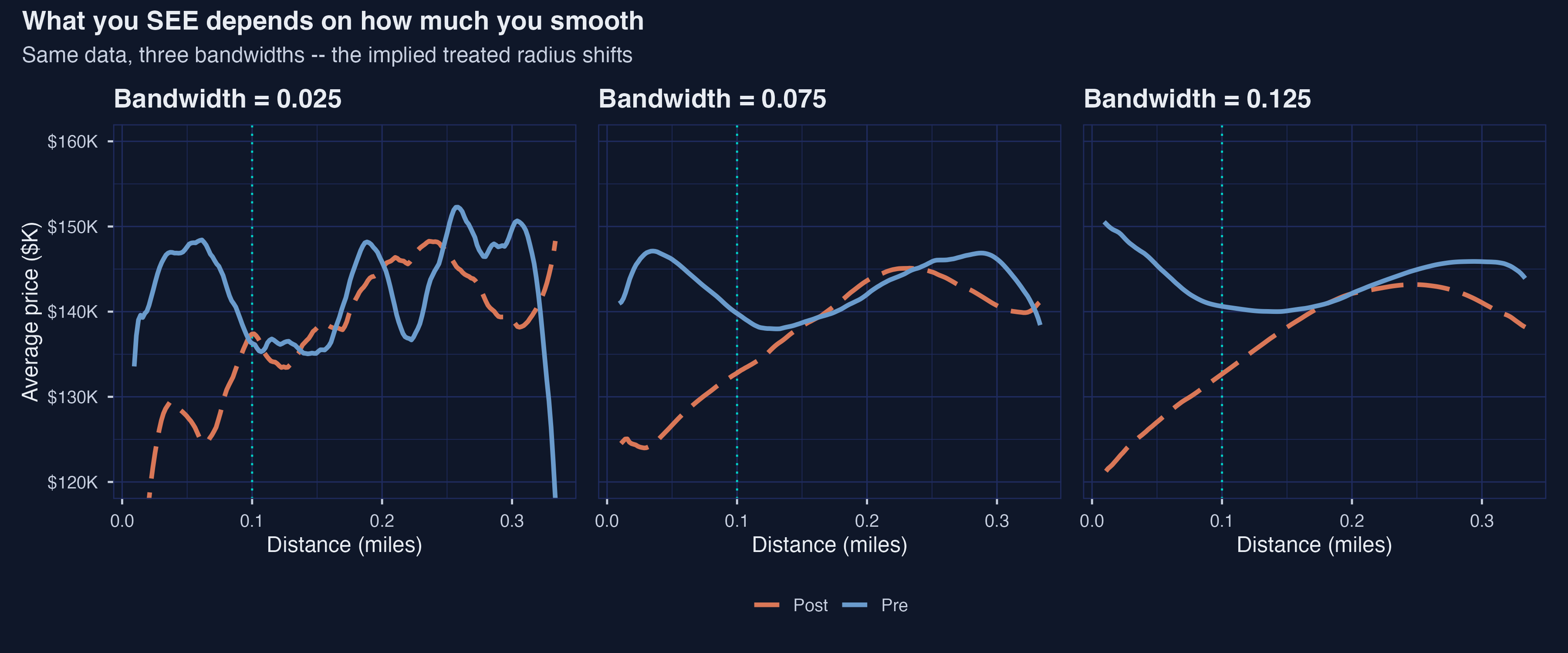
Same data, three smoothing bandwidths — the implied treated radius shifts from ~0.10 mi (bw 0.025) to ~0.20 mi (bw 0.125).

On the real Linden-Rockoff gradient: bandwidth 0.025 suggests a treated radius near 0.10 mi; 0.075 stretches it to ~0.15; 0.125 to ~0.20. Same data, three smoothers, three visual “answers” about how far the effect reaches. This is the bandwidth-version of ring-choice fragility — the case for not picking a cutoff by inspection.

The Resolution

Act III

On real data, the ring DiD says homes inside 0.1 mile drop 5.78%

−5.78%

parametric ring DiD, ATT at 0.1 mi · SE 0.0225 · 95% CI \([-10.4\%,\, -1.5\%]\) · \(n = 9{,}029\)

9,092 North Carolina sales within 1/3 mile of an offender; 1,093 inside the 0.1-mi treated ring. close_post_move coefficient −0.0595 log-points, neighborhood-clustered SE 0.0225, CI strictly excluding zero. Butts reports “about 7.5%” — our −5.78% sits within rounding and inside our own ring-choice spread. Qualitative agreement, headline within reach.

Redraw the radius and the headline wobbles 52% — the sign holds, the magnitude doesn’t

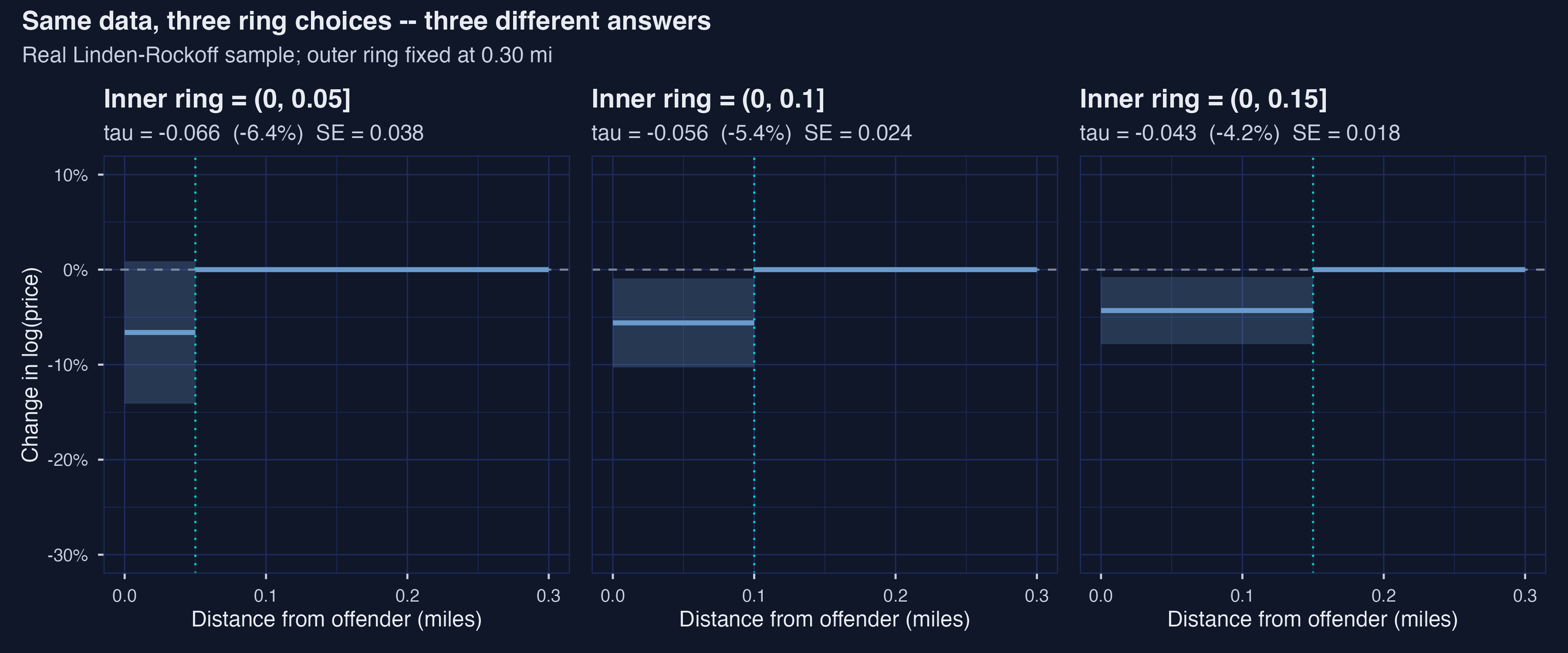
Three inner-ring cutoffs on the same data: ATT moves from −6.40% (0.05 mi) to −4.21% (0.15 mi) — a 52% relative spread driven entirely by the cutoff.

Cutoff	ATT (%)	95% CI
0.05 mi	−6.40%	\([-14.1\%, +0.9\%]\)
0.10 mi	−5.45%	\([-10.3\%, -0.9\%]\)
0.15 mi	−4.21%	\([-7.8\%, -0.8\%]\)

Outer ring fixed at 0.3 mi; only the inner cutoff moves. ATT swings from −6.40% to −4.21% — a ~52% relative spread, pure researcher choice, zero sampling noise involved. Sign is stable, every estimate distinguishable from zero. But a reader shown only one number gets a noticeably different impression. As Butts puts it: “the choice of 0.1 miles is an untestable assumption.”

Let the curve flex and the closest 300 feet drop 20.6% — twice the parametric average

−20.6%

nonparametric bin 1 (first ~300 ft) · sample-weighted ATT inside 0.1 mi \(= -12.4\%\), about \(2.1\times\) the parametric −5.78%

binsreg carves the inner sample into 23 bins. Bin 1 (~first 300 ft) = −20.6% [−34.0, −12.1]; bin 2 = −15.2%; by bin 4 (~0.10 mi) it is +0.6%, indistinguishable from zero. Sample-weighted inside-0.1-mi ATT = −12.4%, ~2.1× the parametric −5.78%. No disagreement — the parametric coefficient averages a steep near-effect with a near-zero outer edge; the curve reveals the concentration the average hides.

The data-driven cutoff lands at 0.094 mi — validating the radius Linden & Rockoff guessed

Parametric

• one number per radius
• −5.78% at 0.1 mi
• magnitude conditional on \(\bar d\)
• 52% spread across choices

Nonparametric

• a whole \(\hat\tau(d)\) curve
• −20.6% in the closest bin
• crosses zero at \(d \approx 0.094\) mi
• the cutoff is an output, not an input

The reconciliation: same data, different questions. The nonparametric curve crosses zero between bins 3 and 4 (≈0.094 mi) — strikingly close to the 0.1-mi cutoff Linden & Rockoff chose by eyeballing the smoothed gradient. The data-driven estimator endorses their guess as an output of the analysis, not an assumption fed into it. Best evidence the two approaches are complementary.

Does the nonparametric estimator make this causal? No — assumptions still carry the weight

Objection. A flexible, data-driven estimator must give the “true” causal effect — no researcher choice, no bias.

Response. Flexibility removes the cutoff choice, not the identifying assumptions. The ATT is identified only under local parallel trends and no anticipation — both untestable in this cross-section. binsreg discovers the shape; it cannot manufacture identification.

Steelman, don’t strawman. The nonparametric estimator disciplines the cutoff but leaves the assumptions untouched: no formal pre-trends test in cross-section, no test of no-anticipation. The oscillation around zero past 0.1 mi is suggestive, not dispositive. Butts and Linden-Rockoff both disclaim a definitive causal reading — the post adopts the same humility.

Report both numbers: the average is correct, the curve is the whole story.

The single takeaway. −5.78% (parametric average) and −20.6% (closest bin) are both correct — they answer slightly different questions. Reporting only one paints a correct but partial picture of a hyper-local externality. Let the data trace the curve, then summarize honestly.