Dynamic Panel BMA

Which factors truly drive economic growth — once reverse causality is handled?

0.990population — robust across every prior

0.92lagged GDP — slow convergence

512models averaged

Carlos Mendez

Nagoya University (GSID)

June 11, 2026

The Tension

Act I

A government asks: which of 9 levers actually accelerates growth?

You advise a government with a panel of 73 countries over four decades and nine candidate drivers — investment, education, trade, population, life expectancy, and more.

But today’s GDP may itself cause investment and trade. Can you trust a regression that assumes the arrow only runs one way?

This is the framing of the whole tutorial. Fast-growing countries also invest, trade, and educate more — so cross-sectional growth regressions, which assume strict exogeneity, can confidently point to the wrong variables. Reverse causality contaminates the answer before model uncertainty even enters.

With 9 candidates there are 512 models — and no reason to trust just one

Build one model with all 9 regressors? Drop trade? Use only investment and education? With 9 candidates there are \(2^9 = 512\) possible specifications.

Bayesian Model Averaging refuses to pick one. It averages all 512, weighting each by how well it fits — so the conclusion never rests on a single lucky specification.

BMA replaces “which model is right?” with “how much does each model deserve to be believed?” Each specification gets a posterior weight; the reported coefficients are weighted averages across the whole 2^K space. The companion cross-sectional post averaged 4,096 models of CO2 emissions; here we move to dynamic panel data.

Where we’re going

• Why cross-sectional BMA misleads when regressors are endogenous
• The dynamic panel fix: lagged GDP + entity and time fixed effects
• BMA over all 512 models — Posterior Inclusion Probabilities (PIPs)
• Stress-testing every PIP against three different priors
• Jointness: which determinants are complements

The Investigation

Act II

Cross-sectional BMA assumes strict exogeneity — and growth data breaks it

Judge a runner’s program by their finish time — but faster runners also chose better programs. Did the program cause the speed, or the speed attract the program?

That is reverse causality. Countries that grow faster invest, trade, and educate more — so a model averaged over biased specifications averages over biased answers.

The model-averaging machinery works perfectly; the individual models it averages are biased. The fix is to control for last period’s GDP — by conditioning on where a country was, we isolate which new factors push it forward and break the feedback loop.

The Solow model makes lagged GDP unavoidable, not optional

\[\ln y_{it} = \alpha \ln y_{i,t-1} + \beta' x_{it} + \eta_i + \zeta_t + v_{it}\]

The convergence prediction puts last period’s GDP on the right-hand side. The persistence \(\alpha\) measures how slowly countries approach their steady state.

Omitting \(\ln y_{i,t-1}\) assumes \(\alpha = 0\) — instantaneous convergence, which the data flatly rejects.

α close to 1 means slow convergence (countries stay near their current income for a long time); α close to 0 means fast. The lagged dependent variable is not an ad hoc add-on — it falls straight out of the Solow beta-convergence equation. Entity effects absorb geography and institutions; time effects remove global shocks.

Weak exogeneity buys realism: past feedback allowed, current shock forbidden

Strict exogeneity (cross-section)

• one time snapshot
• no lagged outcome
• no fixed effects
• regressors clean at all times

Weak exogeneity (dynamic panel)

• four decades of panel
• lagged GDP included
• entity + time effects
• only the current shock \(v_{it}\) ruled out

Weak exogeneity allows past GDP growth to influence current investment — the realistic feedback loop — while requiring only that today’s idiosyncratic shock v_it does not simultaneously move today’s investment. Much weaker than strict exogeneity, and exactly what growth data needs.

Estimate all 512 models by marginal likelihood, not R-squared

data_std <- feature_standardization(economic_growth,
              excluded_cols = c(country, year, gdp))  # mean 0, sd 1
# demean by year → remove time fixed effects, then estimate every model
full <- optim_model_space(df = data_prepared,
          dep_var_col = gdp, timestamp_col = year,
          entity_col  = country, init_value = 0.5)
bma_results <- bma(full, df = data_prepared, round = 3)

Marginal likelihood scores each of 512 “recipes” — rewarding fit, penalizing needless complexity.

Unlike R-squared, which always rises when you add variables, the marginal likelihood integrates out parameter uncertainty and penalizes complexity — a 9-regressor model that barely beats a 5-regressor one scores lower. The package ships a precomputed full_model_space so the several-minute optimization can be skipped.

Kitchen-sink FE finds 6 of 10 significant — but the verdict reshuffles

Regressor	Coef.	p-value	Sig. 5%?
lag GDP	0.619	0.000	yes
trade openness	0.120	0.002	yes
education	0.016	0.632	no
life expectancy	0.115	0.637	no

Drop one variable and the significance pattern changes — this fragility is what BMA is built to fix.

The kitchen-sink fixed-effects model commits to one specification. Its lagged-GDP coefficient (0.619) is well below the BMA posterior mean (0.919) — multicollinearity among 9 regressors pulls it down. R-squared is 0.988 on 292 observations. BMA replaces the binary significant/insignificant verdict with a continuous probability scale.

BMA grades each variable on a continuous PIP scale — population leads at 0.990

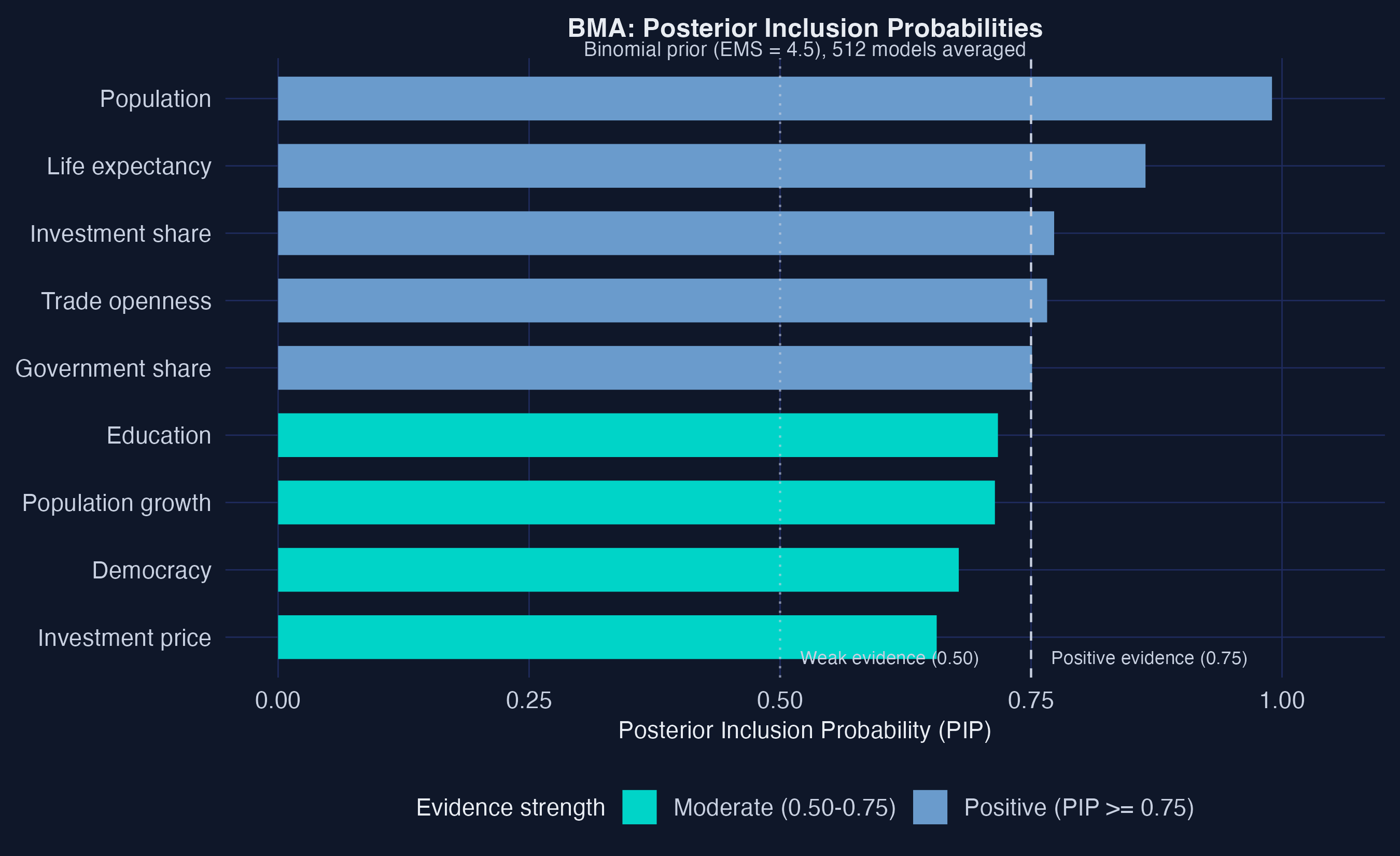
Posterior Inclusion Probabilities, all 9 regressors, sorted with the 0.75 and 0.50 threshold lines.

The PIP is the share of posterior mass in models that include the variable — a “batting average.” Population dominates at 0.990 (strong evidence), life expectancy at 0.864. Five variables clear the 0.75 positive-evidence threshold; the rest sit in the 0.50–0.75 moderate zone. No variable falls below 0.50 — the data supports relatively large models.

Population is the single most robust determinant: PIP = 0.990

0.990

Population PIP under the binomial prior — appears in virtually every high-quality model

On Raftery’s classification 0.990 is “strong” evidence — just short of the 0.99 “very strong” cut. Population is followed by life expectancy at 0.864 and investment share at 0.773. Every one of the 9 candidates exceeds 0.65, so this is a story about which variables are most robust, not which clear a yes/no bar.

The data concentrates posterior mass on a few large models

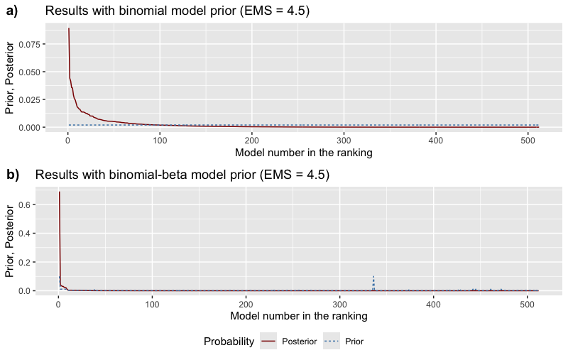
Prior (flat, dashed) vs posterior (concentrated, solid) probability across all 512 models.

The prior is nearly flat; the posterior spikes on a handful of models while most receive negligible weight. That concentration is the signature of informative data — 73 countries over four decades carry enough information to strongly favor certain specifications.

The posterior wants big models — expected size jumps from 4.5 to ~7

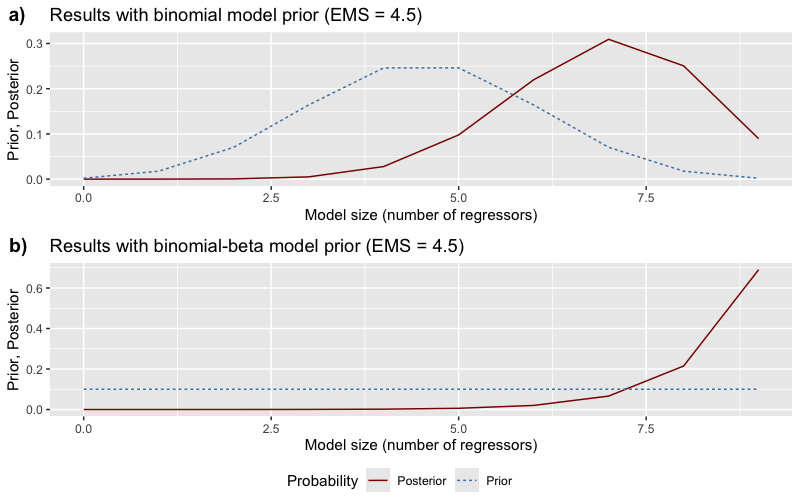
Prior vs posterior distribution over model sizes (regressors excluding the lagged outcome).

The binomial prior centers on 4–5 regressors (EMS = 4.5); the posterior shifts to 6.908. Under the binomial-beta prior it reaches 8.556 — the data wants nearly all 9 candidates. Consistent with every variable having PIP above 0.65: the data sees signal almost everywhere.

The best single model carries only 8.9% of the mass — no model is “the” model

8.9%

Posterior weight on the top-ranked specification; the other 91% spreads across hundreds of nearby models

The top model includes all 9 regressors (PMP = 0.089); the next seven each drop exactly one variable — a “kitchen sink minus one” pattern. Population and life expectancy are never dropped across the top 8, matching their high PIPs. This is precisely why averaging beats selecting: betting on one specification ignores 91% of the evidence.

Posterior coefficients: population and life expectancy clear zero cleanly

Posterior means with approximate 95% credible intervals (\(\text{PM} \pm 2\cdot\text{PSD}\)) for all 9 regressors.

Population and life expectancy have the largest positive posterior means with intervals away from zero. Democracy is clearly negative. Education and government share straddle zero — reflecting sign instability. BMA’s intervals are wider than ordinary confidence intervals because they absorb variation across specifications, not just within one.

Population’s coefficient is tight, positive, and centered near 0.12

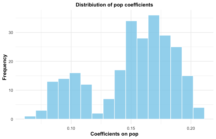
Posterior coefficient distribution for population across all 512 models, weighted by model probability.

A tight, entirely positive distribution centered around 0.12 — strong and stable evidence for a positive effect on growth. This is the visual companion to population’s 0.990 PIP: not just frequently included, but consistently signed and precisely estimated.

A skeptical prior is the real test — only population and life expectancy survive it

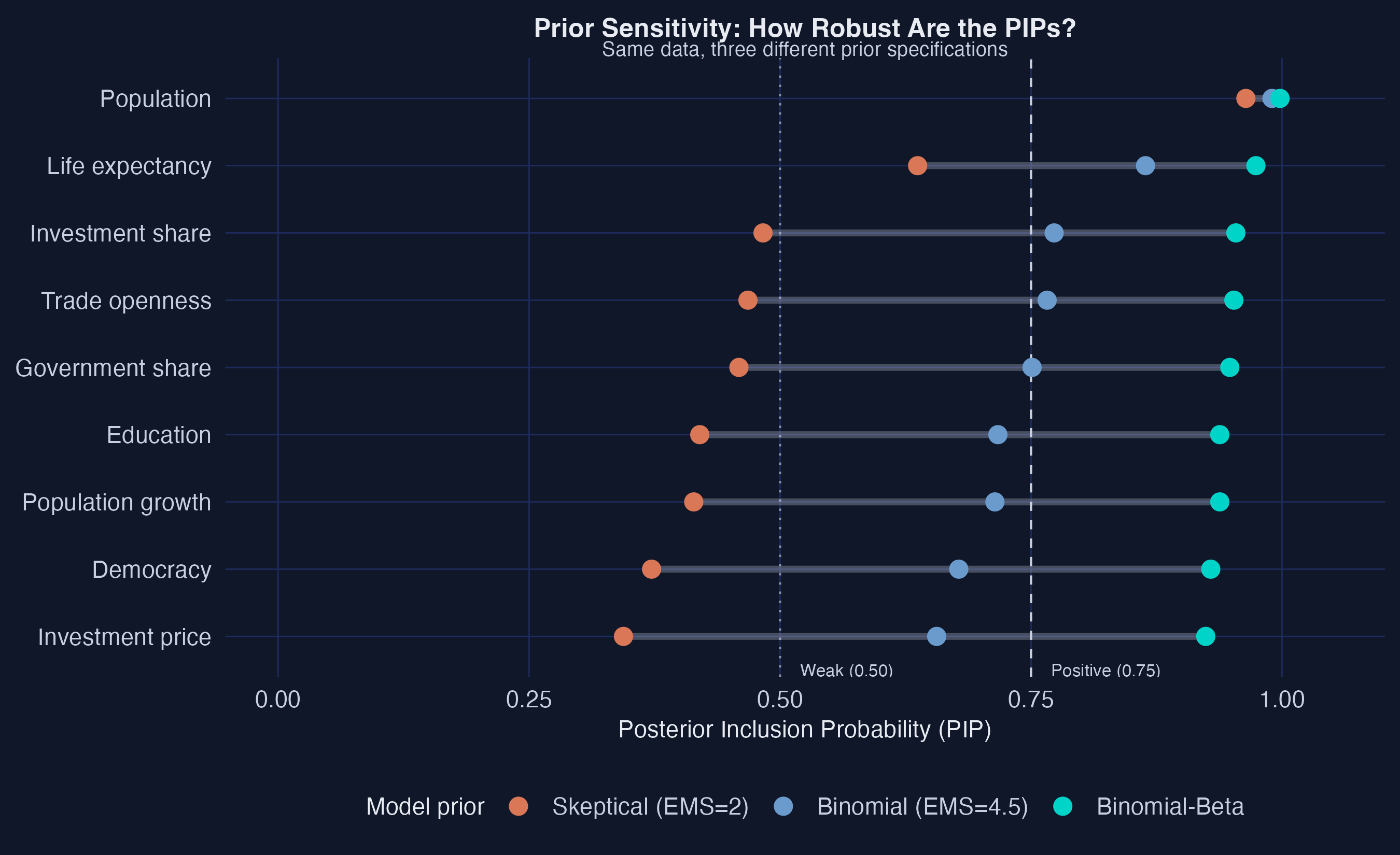
PIPs under three priors (skeptical EMS=2, binomial, binomial-beta). Segment width = sensitivity.

Segment width shows how much each PIP moves across priors. Population is rock-solid (0.964–0.998); life expectancy moderately sensitive (0.637–0.974). Under the skeptical EMS=2 prior, investment share collapses from 0.773 to 0.483 and democracy to 0.372 — only pop and lnlex stay above 0.5. The headline: robustness means surviving the prior that wants you gone.

A dilution prior penalizes redundant controls — the ranking holds

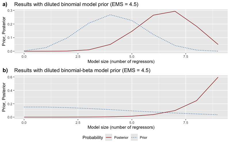
Model sizes under the dilution prior (penalizing correlated regressors); expected size falls 6.91 → 6.53.

The dilution prior multiplies each model’s prior by the determinant of its regressors’ correlation matrix — near-duplicate variables get pushed toward zero. PIPs drop modestly (ish 0.773 → 0.718) and expected size falls from 6.91 to 6.53, but the ranking is unchanged: pop and lnlex stay on top. A clean robustness check against multicollinearity inflation.

Population and life expectancy are complements, not substitutes — jointness 0.711

Complements everywhere

• All HCGHM pairs are positive
• Strongest: \(\text{pop} \times \text{lnlex} = 0.711\)
• \(\text{pop} \times \text{ish} = 0.530\)
• \(\text{pop} \times \text{opem} = 0.517\)

Reading it

• No substitution detected
• Determinants add distinct stories
• Investment price is the loner

Jointness measures whether two regressors appear in models together (complements) or apart (substitutes). Every pair here is a complement — population and life expectancy most strongly at 0.711, meaning they tell additive, non-overlapping growth stories. Under the binomial-beta prior the values climb to 0.944 because larger models make co-appearance more likely.

The Resolution

Act III

GDP is highly persistent — only ~8% of the steady-state gap closes per decade

\[\alpha \approx 0.92 \;\Rightarrow\; \text{convergence speed} = 1 - \alpha \approx 0.08 \text{ per decade}\]

The lagged-GDP coefficient near 0.92 means a country’s income is dominated by its own past — convergence to its steady state is a slow crawl.

That persistence absorbs the cross-sectional variation, leaving fewer variables with independent power.

The kitchen-sink FE coefficient (0.619) understates persistence; the BMA posterior mean is 0.919–0.943 depending on prior. Strong persistence is exactly why dynamic panel BMA reshapes the landscape of “robust” determinants relative to cross-sectional BMA — much of what looked causal was just inertia.

Controlling for reverse causality leaves population and public health standing

Determinant	Bin.	Bin-Beta	EMS=2	Verdict
population	0.990	0.998	0.964	Robust
life expectancy	0.864	0.974	0.637	Robust
investment share	0.773	0.954	0.483	Sensitive
democracy	0.678	0.929	0.372	Sensitive

Robust = PIP above 0.5 even under the skeptical prior. Only two determinants qualify.

This is the payoff table. Investment and trade look promising under the default prior but become ambiguous under EMS=2. Education and democracy — despite intuitive appeal — are fragile. For a policymaker, population dynamics and public health are the levers with the strongest evidence across all modeling assumptions.

Does dynamic panel BMA make these causal? No — it disciplines, it doesn’t identify

Objection. Adding a lagged outcome and fixed effects can’t manufacture causal identification.

Response. Correct. The estimates are consistent only under weak exogeneity — current regressors uncorrelated with the current shock. If contemporaneous feedback is strong, bias remains. BMA handles model uncertainty and reverse causality through persistence; it does not relax the identifying assumption.

Steelman, don’t strawman. Weak exogeneity is weaker than strict, but it is still an assumption — a same-period GDP shock that immediately moves investment would break it. The contribution is robustness of which determinants survive, not a clean causal effect for any one of them.

Once reverse causality is handled, only population and public health hold up.

The single takeaway. Across 512 models and three priors, controlling for GDP’s persistence dissolves most “robust” growth determinants — leaving population dynamics and life expectancy as the two levers with evidence that survives even a skeptical prior.