Who Are My Neighbors?

Bayesian estimation of spatial weight matrices — and what changes when you stop assuming

8,010links estimated, not assumed

ρ = 0.713reproduced to 5 decimals

2.1×spillover vs own-region effect

Carlos Mendez

Nagoya University (GSID)

July 31, 2026

The seating chart you were handed

You have the full transcript of a conference dinner: who laughed at which joke, who fell silent when.

You do not have the seating chart.

Spatial econometrics hands you the chart first — drawn from shared borders or straight-line distance — and asks you to trust it.

Open with the analogy, not the equation. The audience needs to feel the problem before seeing the machinery.

The Tension

Every spillover estimate is conditional on a matrix somebody chose

\[y_t = \rho W y_t + Z_{t-1}\beta + \varepsilon_t\]

• \(W\) says who is whose neighbour
• \(\rho\) says how strongly neighbours matter
• \(W\) is normally assumed, never estimated

If the map is wrong, every number downstream is wrong.

Emphasise: this is not a small auxiliary choice. It is upstream of everything.

On this data, contiguity needs ten arbitrary decisions

Ten of ninety European NUTS-1 regions have no queen-contiguity neighbour at all:

Cyprus · Malta · Aegean islands · Canarias · Åland · Corse · Sicily & Sardinia · Azores · Madeira · Ireland

Each must be patched by hand before a contiguity model will even run — and those patches are invisible in the results table.

This is the single most persuasive slide for a sceptical audience. The “standard” approach already required ten undocumented judgement calls.

The Investigation

Treat all 8,010 links as unknown parameters

	Assumed \(W\)	Estimated \(W\)
\(\rho\), \(\sigma^2\)	2	2
Slopes	4	4
Off-diagonal cells	0	8,010
Total unknowns	6	8,016
Observations	1,710	1,710
Obs per unknown	285	0.21

4.7 parameters per observation. The likelihood alone cannot do this.

The prior is not a technicality — it is the method

\[p_{ij} \;\propto\; \omega_{ij} \;\times\; m(k_i)\]

Where links can be × how many there are.

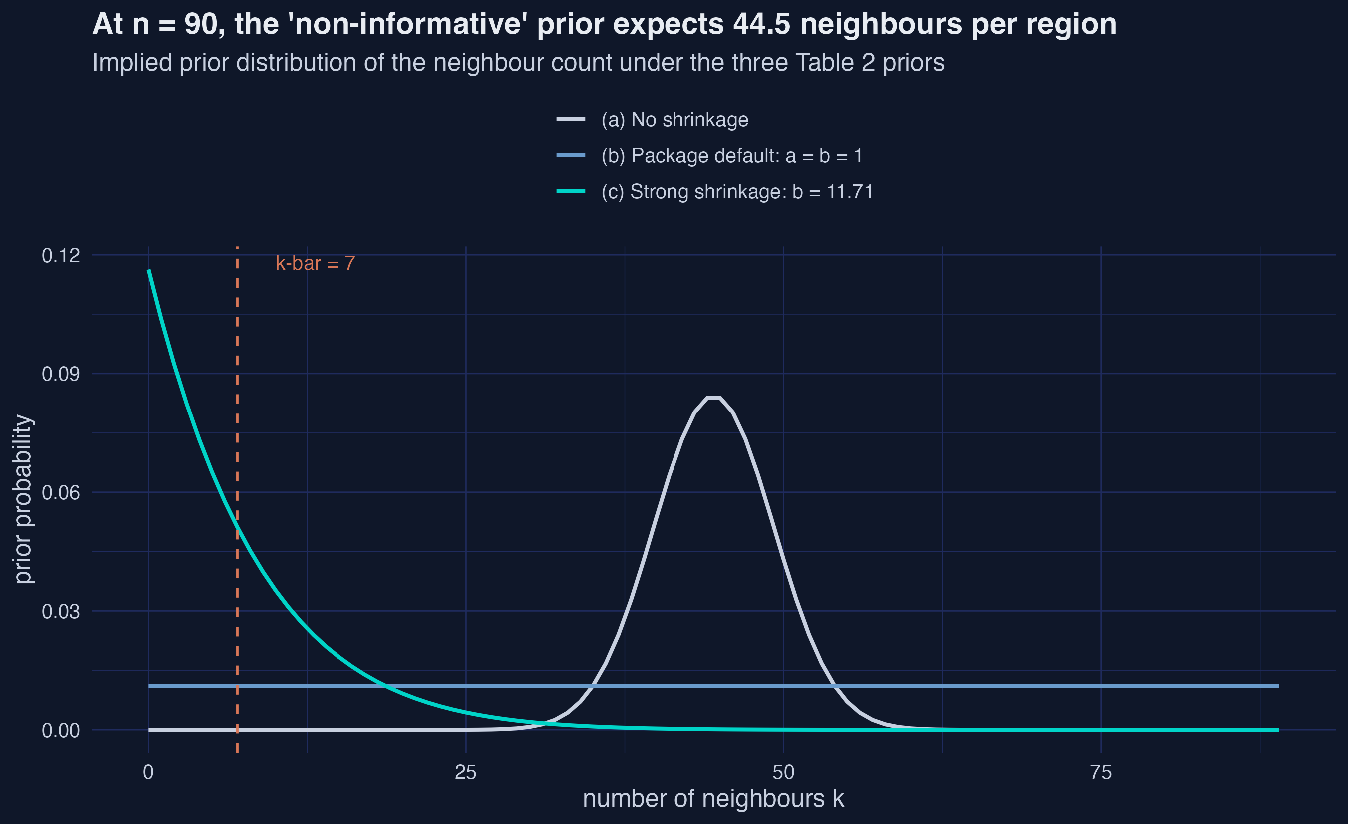
The trap: a “non-informative” flat prior on the neighbour count implies an expectation of 44.5 neighbours per region — every region wired to half of Europe.

The paper writes these hyperparameters with underbars. Dropped here for legibility; the two factors are what matter. Next slide shows what the “non-informative” choice actually asserts.

“Non-informative” means half of Europe

Grey bell centred at 44.5 is the flat prior. Teal spike at 7 is the anchored one. Same word, opposite belief.

One link at a time

A link is on or off, so conditional on everything else there are only two states to score:

\[p(\omega_{ij} \mid \Omega_{-ij}, \cdot, \mathcal{D}) \sim \text{Bernoulli}\left(\frac{\bar{p}^{(1)}_{ij}}{\bar{p}^{(0)}_{ij} + \bar{p}^{(1)}_{ij}}\right)\]

Score both, normalise, flip a weighted coin. Repeat 8,010 times per sweep.

Sherman-Morrison rank-one updates make each flip cheap instead of an \(O(n^3)\) determinant.

Piano-tuning analogy: never solve the whole instrument, fix one string given the others.

First, check it on a network we built ourselves

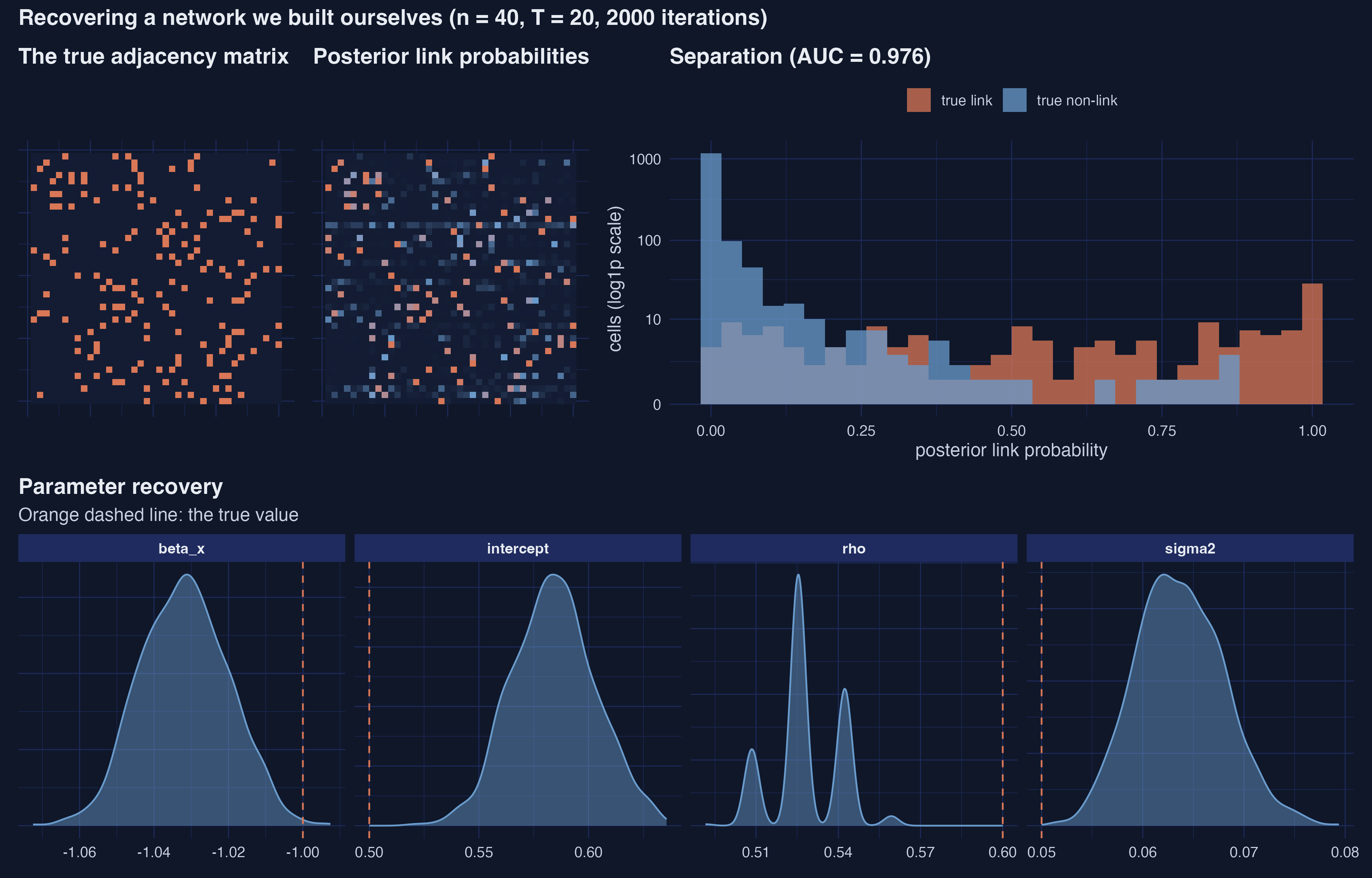
AUC 0.976 · 95.3% of 1,560 cells classified correctly

Driving test where you placed the cones. Build trust before spending it on real data.

But the intervals are not calibrated

	True	Estimate	95% interval	Covered?
\(\rho\)	0.600	0.528	[0.509, 0.542]	no
\(\sigma^2\)	0.050	0.064	[0.056, 0.073]	no
slope	−1.000	−1.032	[−1.053, −1.009]	no

Sparsity biases the network sparse, and \(\rho\) down with it. Autocorrelation narrows the intervals.

Trust the structure. Hedge the intervals.

The Resolution

The published table reproduces exactly

Quantity	Paper	Ours	Verdict
\(\rho\)	0.71322	0.71322	exact
log initial GVA	−0.01692	−0.016922	exact
share high education	0.00044	0.000441	exact
av. indirect, initial GVA	−0.03972	−0.039723	exact

12 of 12 quantities exact to the five decimals printed — same seed, same package version, same RNG, same BLAS.

The model reconstructed national borders

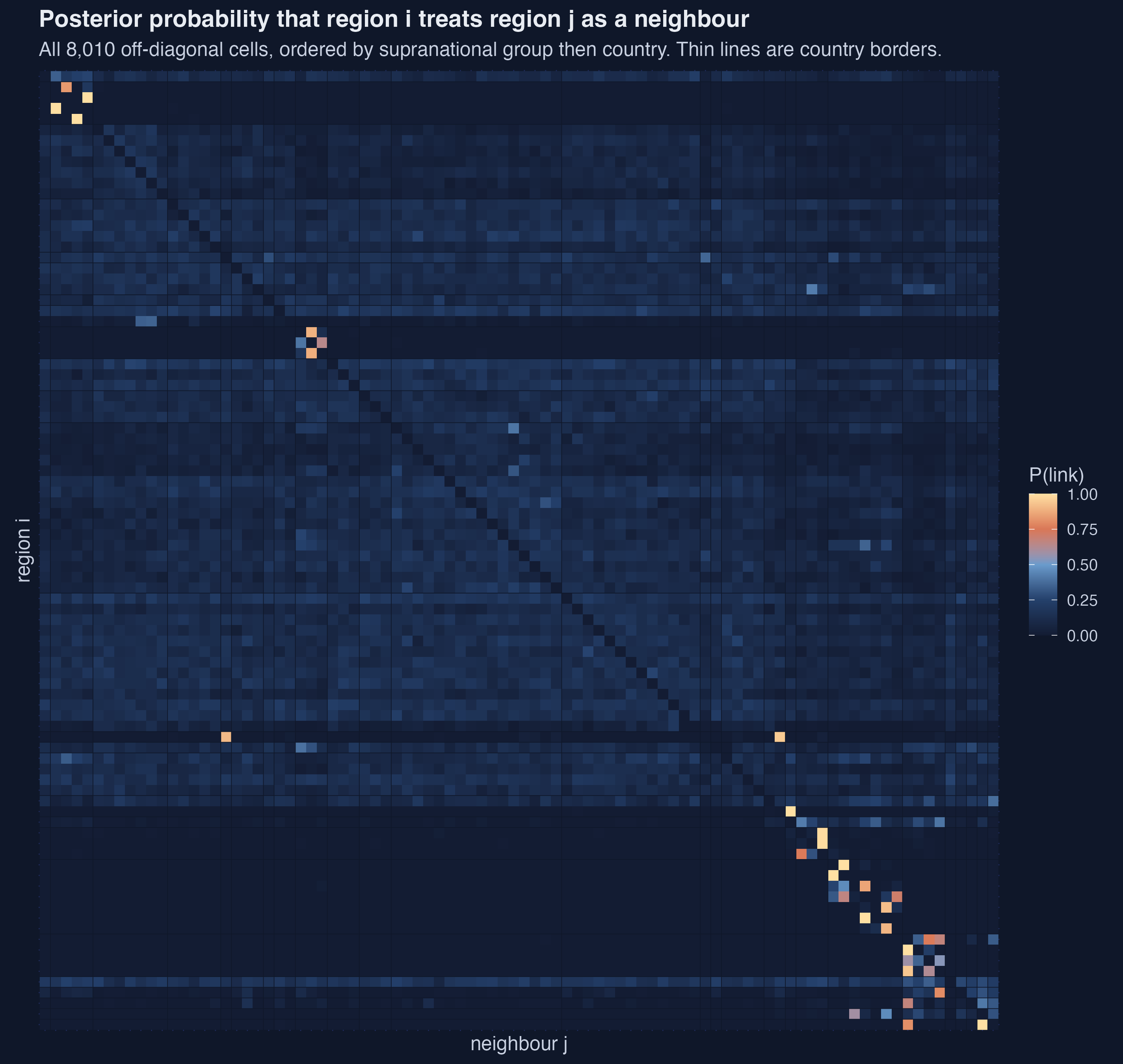
Regions place 35.6% of their neighbourhood weight on compatriots.

Chance would give 7.1%.

Nothing in the specification mentions countries — the model saw only growth rates, initial productivity and two education shares.

Same country beats shared border

Comparator	AUC	Share of top links
Same country	0.753	30.2%
Queen contiguity	0.698	17.2%
7-nearest neighbours	0.631	23.9%

Strongest estimated links average 921 km, against 1,331 km for a random pair — geography still matters, just far less than nationality.

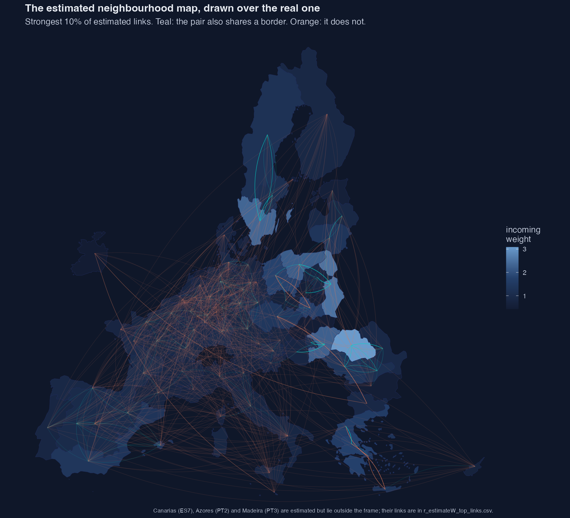
Look at the map

Teal — the pair also shares a border.

Orange — it does not.

Long orange arcs dominate: Bulgaria to Czechia, Iberia to the Baltic, Greece to Ireland.

If the estimated network were essentially contiguity, this would be a mesh of short teal arcs hugging borders.

Three maps, three answers

	Estimated	Queen	7-NN
\(\rho\)	0.713	0.607	0.719
High education, total	0.00153	0.00066	0.00074
Indirect ÷ direct	2.11	1.20	2.20

Every sign survives. Every magnitude moves.

The data-chosen map more than doubles the total education effect.

Why that matters for policy

A region raising tertiary attainment generates roughly twice as much growth outside its borders as inside them.

Whoever funds the universities captures about a third of the return.

Under contiguity that ratio is 1.20, not 2.11 — the difference between “most of the return leaks away” and “about half does”.

Different co-funding decision.

What this cannot tell you

A posterior probability of 1.0 on Bulgaria → Czechia means residual co-movement is better explained with that link than without it, given a prior expecting seven neighbours.

It does not mean trade, commuting, or FDI.

With \(T = 19\), genuine transmission and shared exposure to common shocks are indistinguishable.

Do not let anyone leave the room thinking this is a causal network.

Honest limits

• ESS(\(\rho\)) = 26.5 out of 100 retained draws; Geweke \(z = -3.74\)
• Posterior means are stable across chains and budgets
• Posterior SDs, intervals and link rankings are not
• With 100 draws a link probability is quantized to 0.01
• Practical ceiling: about 300 regions
• \(\underline{k} = 7\) is a researcher choice — report a sweep, not a number

The map is a parameter

Every spatial result you have read is conditional on a neighbourhood map somebody chose before the analysis began.

It does not have to be.

Full tutorial, code and replication bundle: https://carlos-mendez.org/post/r_estimatew/