Bayesian Spatial Synthetic Control

California’s Proposition 99, three estimators, and a Nevada-sized spillover

−18.46ATT · packs per capita per year

−3.75Nevada spillover · SUTVA fails

0.223spatial autocorrelation rho

Carlos Mendez

Nagoya University (GSID)

June 11, 2026

The Tension

Act I

Two assumptions decide whether you trust the most-studied policy in econometrics

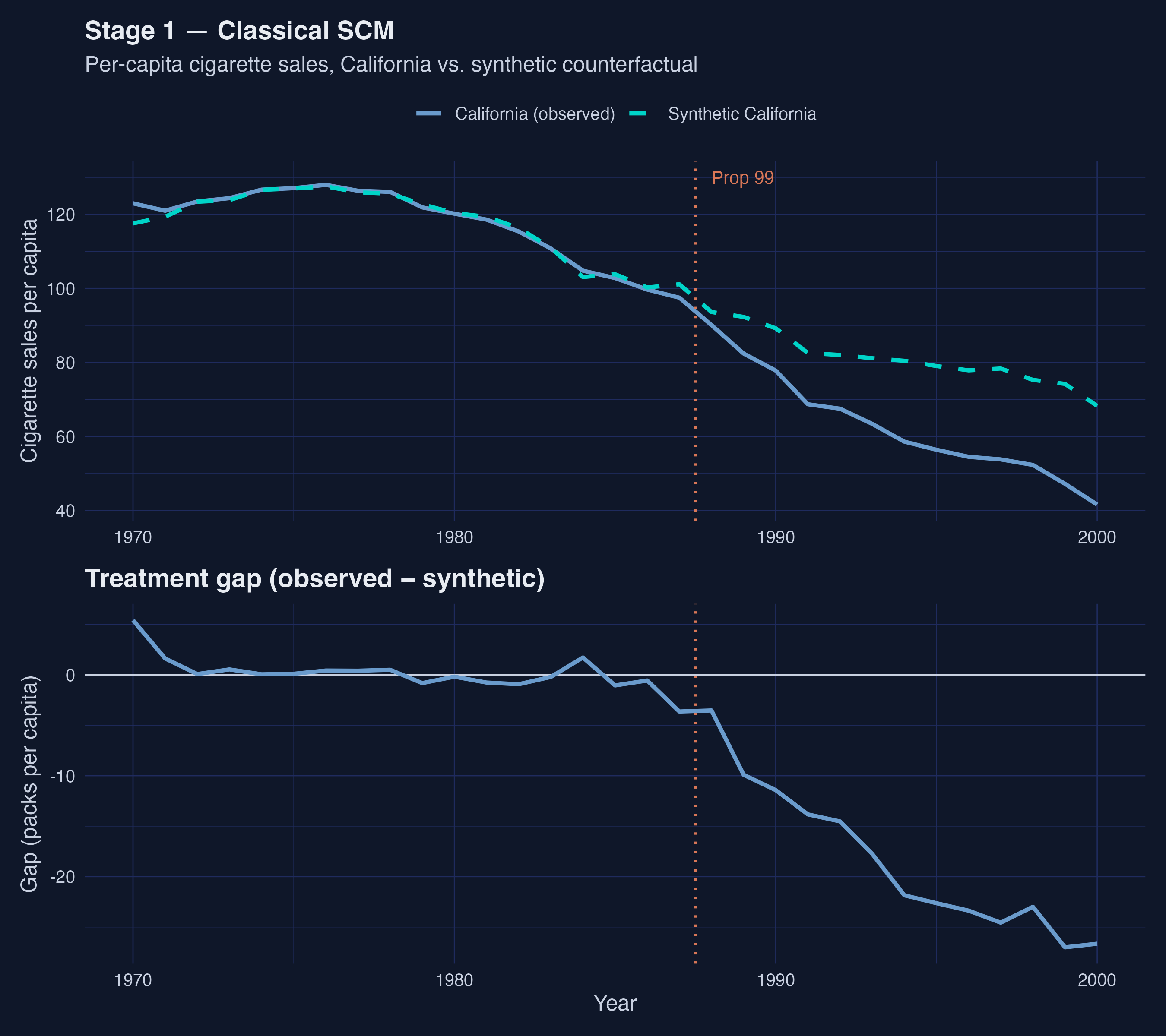
Prop 99 raised California’s cigarette tax 25 cents in 1988. The classic answer — a 25–30 pack drop — has been quoted for 20 years.

But it rests on two quiet assumptions: donor weights live on a sparse simplex, and donor states are unaffected by California’s policy. What if both are wrong?

This is the central tension. Classical SCM gives a clean headline, but the simplex constraint may manufacture its four-donor sparsity, and SUTVA may be violated by Californians driving to Nevada for cheaper cigarettes. We will test both — and reject one.

Same data, three estimators, one ATT — but the donor pool quadruples

ATT stays −18 to −16 packs/capita across all three estimators; active donors climb 4 → 23 → 27.

Spoiler figure. Don’t explain the gap yet — just plant that the headline ATT survives all three specifications, while the synthetic California’s composition does not. We earn each estimator in Act II and return to this picture.

Where we’re going

• The case: California, Prop 99, and the SUTVA problem
• Three nested estimators — classical → horseshoe → spatial
• The ATT (the estimand) and how its credible interval moves
• The spillover that proves SUTVA is empirically false

The Investigation

Act II

The estimand is the ATT for one treated unit: California

\[\mathrm{ATT} = E\big[Y_i(1) - Y_i(0) \mid D_i = 1\big]\]

With a single treated unit, the ATT is the gap between observed California and a counterfactual California, averaged over 1988–2000.

Every stage targets the same ATT — only the way it builds the counterfactual California changes.

Be explicit about the estimand: this is the average treatment effect on the treated, not on the population. We never observe untreated California after 1988, so we construct a synthetic twin from donor states. The whole deck is about how that twin is built.

The lab: a balanced 39-state panel, 1970–2000, 1,209 rows

• Outcome — per-capita cigarette sales (cigsale)
• Treated — California; treatment switches on in 1988
• Donors — the other 38 states, untreated throughout
• Pre / post — 18 pre-treatment years, 13 post-treatment years

Spatial structure ships with the data: a 38×38 binary contiguity matrix \(W\) among donors, row-normalized before it enters the SAR likelihood.

Three estimators relax one assumption at a time

Stage 1 — Classical

• simplex weights (Abadie 2010)
• SUTVA imposed
• tidysynth

Stages 2–3 — Bayesian

• horseshoe prior on weights
• SAR layer drops SUTVA
• C++ Gibbs samplers

Each arrow weakens an assumption: Stage 1 imposes simplex + SUTVA; Stage 2 relaxes the simplex; Stage 3 also relaxes SUTVA.

The pipeline is the post’s Mermaid diagram, re-expressed as columns: classical → Bayesian horseshoe → Bayesian spatial SAR, then diagnostics and cross-stage comparison. The pedagogical point is what moves between stages.

With zero substantive controls, the simplex picks just four donors

\[\widehat\alpha = \arg\min_\alpha \big\| Y_{1,\text{pre}} - Y_{c,\text{pre}}\,\alpha \big\|^2 \quad \text{s.t.}\quad \alpha_j \ge 0,\ \sum_j \alpha_j = 1\]

The non-negativity-plus-sum-to-one constraint is an implicit regularizer — it pushes most weights to exactly zero.

Read the equation aloud: match California’s pre-treatment sales with a convex combination of donors. The simplex serves interpretability, but it also forces sparsity. Is the four-donor synthetic the data talking, or the constraint?

Classical SCM concentrates 97.5% of the weight on four states

Donor	Weight
Utah	0.327
Nevada	0.255
Montana	0.245
Connecticut	0.148

The other 34 donors are essentially zero — a near-pure four-state synthetic California.

Utah, Nevada, Montana, Connecticut carry 97.5% of the weight. Two questions hang over this: is the sparsity real, and is Nevada — California’s neighbour — contaminated by spillovers? Stages 2 and 3 attack each.

Classical SCM lands the ATT at −18.46 packs per capita

−18.46

ATT, classical SCM (95% bootstrap CI [−22.21, −14.45]) · smaller than Abadie’s −27 because the shipped predictors are leaner

The interval never crosses zero. Our −18.46 is below Abadie’s ≈ −27 because the shipped data only carries cigsale and retprice — no log income, youth share, or beer sales. The pipeline is identical; the inputs are leaner. The qualitative finding survives.

The horseshoe prior keeps zero overwhelmingly likely — yet lets a few donors escape

\[\alpha_j \mid \tau, \lambda_j \sim \mathcal{N}\big(0,\ \tau^2 \lambda_j^2\big), \quad \lambda_j \sim \mathcal{C}^+(0,1), \quad \tau \sim \mathcal{C}^+(0,1)\]

A global scale \(\tau\) pulls everything toward zero; a local scale \(\lambda_j\) lets individual donors break free. The half-Cauchy tails do the rest.

Now the data, not the constraint, decide which donors get non-zero mass.

The horseshoe replaces the simplex with a soft, heavy-tailed regularizer. Most weights hug zero; a handful escape. This is the test of whether the four-donor sparsity was real.

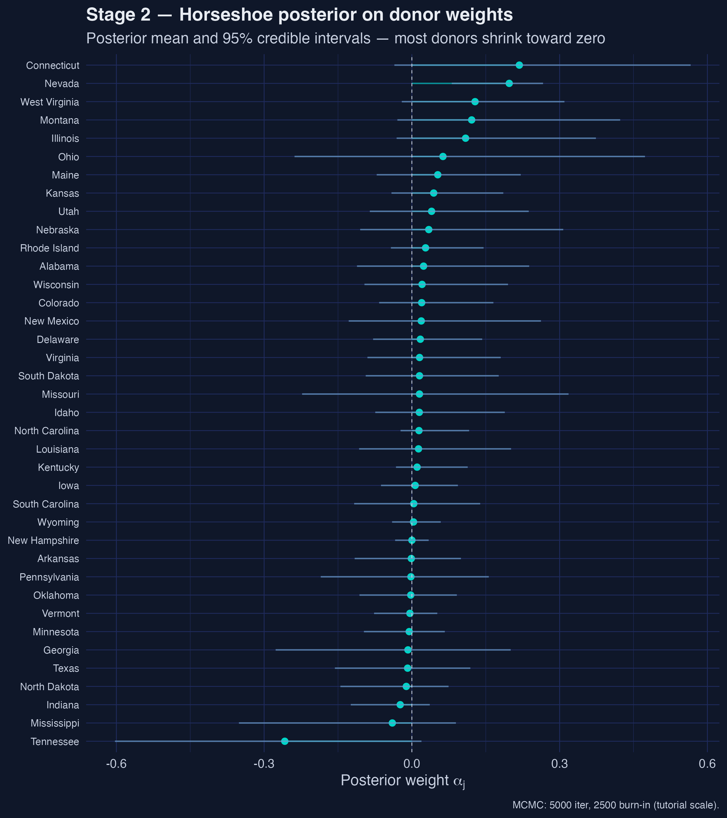
Relax the simplex and the donor pool jumps from 4 to 23 active states

Posterior mean donor weights under the horseshoe, with 95% credible intervals — most hug zero, but only Nevada’s interval clears zero.

23 of 38 donors now carry mean weight above 0.01. Connecticut leads (0.218), but only Nevada’s 95% credible interval [0.081, 0.266] excludes zero. The lesson: classical “sparsity” is partly a constraint artifact — the data do not insist on four donors.

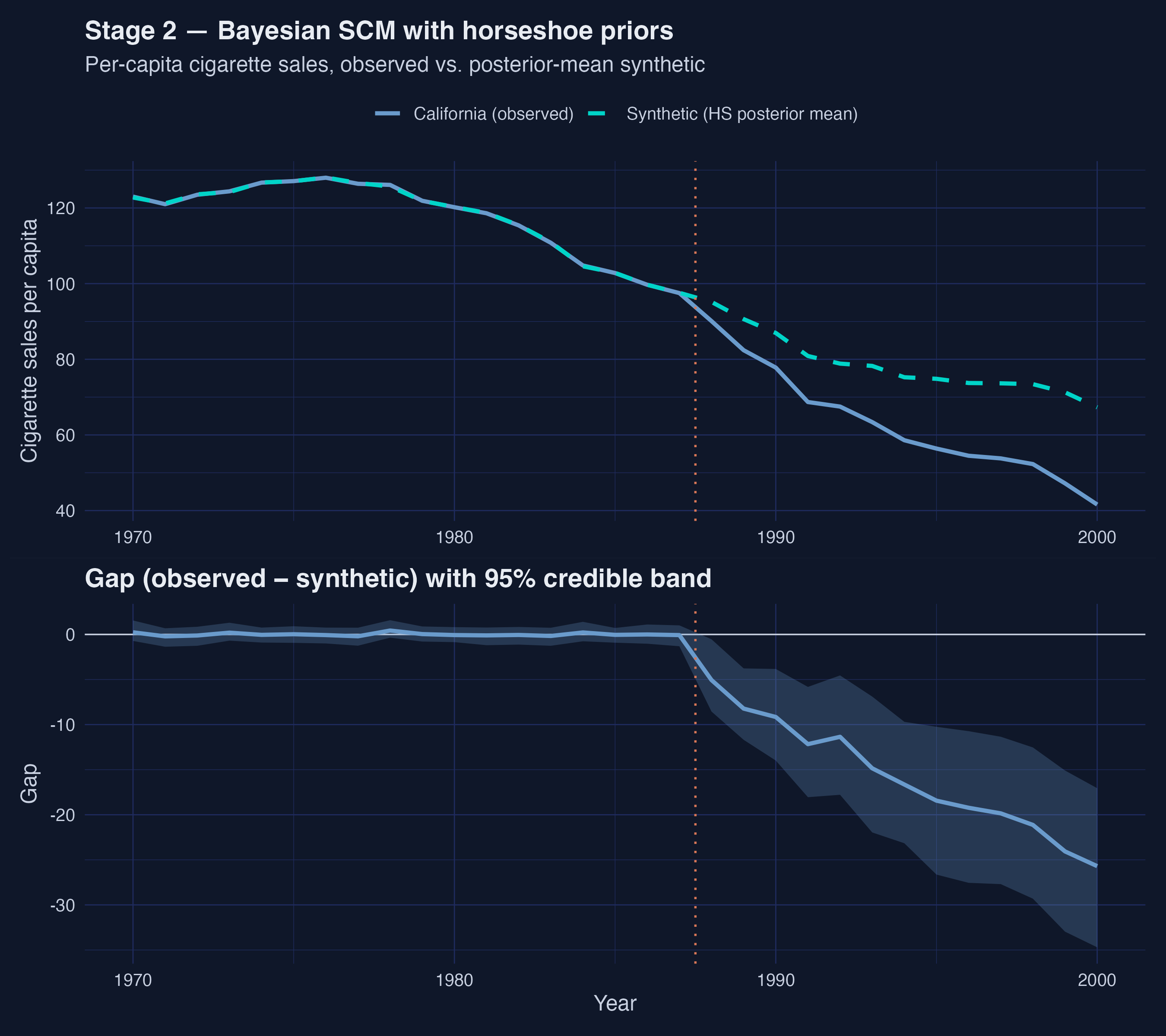
Propagating weight uncertainty widens the band but never reaches zero

California vs horseshoe-posterior-mean synthetic (top) and the gap with a 95% credible band (bottom) — the band widens post-1988 but stays below zero.

ATT moves to −15.84, CrI [−21.76, −9.48] — wider than Stage 1 by design, because the horseshoe carries weight uncertainty into the gap rather than fixing weights at the optimizer’s best guess. Pre-1988 fit is excellent; the post-band reaches ±10 by 1995. Still no zero crossing.

Drop SUTVA: each donor’s sales depend on its neighbours’ sales

\[Y_{c,t} = \rho\, W\, Y_{c,t} + X_{c,t}\beta + Y_c^{\text{lag}}\alpha + \varepsilon_t\]

The spatial lag \(W Y_{c,t}\) is the row-normalized neighbour average; \(\rho\) measures how strongly a state co-moves with its neighbours. When \(\rho = 0\) we recover Stage 2.

If \(\rho > 0\), a donor’s sales are partly its neighbours’ — so Nevada’s post-1988 sales are part of the treatment effect, not the counterfactual.

This is where SUTVA is dropped. The SAR layer lets California’s policy diffuse into adjacent donors through W. The cross-border-shopping literature predicts exactly this for the California–Nevada line.

The Gibbs pipeline runs both MCMCs and the spillovers in one call

w <- as.matrix(california_smoking$w[, 2])    # CA's contiguity row
W <- as.matrix(california_smoking$W[, -1])   # 38x38 donor contiguity
rownames(W) <- colnames(W) <- california_smoking$W$state

fit_sar <- sc_spillover(
  data = panel_df, treated_unit = "California",
  w = w, W = W, y = "cigsale", X = c("retprice"),
  M = MCMC_ITER, burn = MCMC_BURN, seed = SEED)   # horseshoe + SAR

rho_hat    <- fit_sar$rho_hat                  # spatial autocorrelation
att_sar    <- fit_sar$effects$ate_point        # the ATT (estimand)
att_sar_ci <- fit_sar$effects$ate_ci95         # posterior credible interval

sc_spillover runs the horseshoe-alpha and SAR-rho samplers and post-processes the per-state spillovers in one call. The full C++ kernels live in the post’s helpers; here we show the load-bearing lines. The ATT comes from the posterior, with a credible interval — the Bayesian posterior over the effect path is the deliverable.

The posterior puts spatial autocorrelation at rho = 0.223, clearly above zero

0.223

posterior mean \(\hat\rho\) (95% CrI [0.168, 0.272]) · moderate, stable, and bounded away from zero

A 1-unit change in the neighbour-averaged sales moves own sales 0.223 units, controlling for the horseshoe role and retprice. Modest but unambiguously non-zero. The Stage 3 ATT lands at −16.59, between classical and horseshoe — the SAR layer reattributes a sliver of the gap to neighbour diffusion.

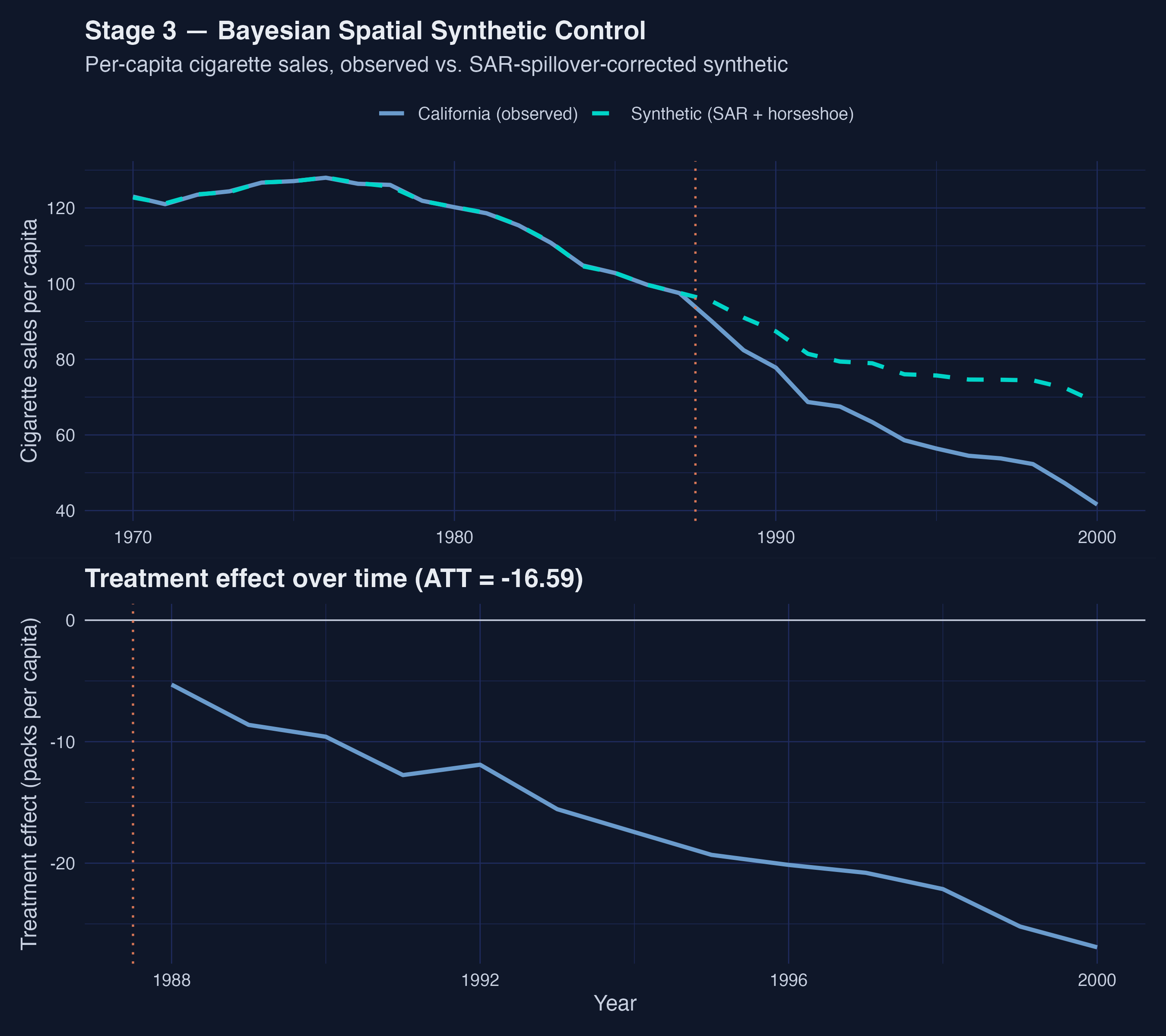
The posterior effect path widens linearly from −5 in 1988 to −27 by 2000

California observed vs SAR-corrected synthetic (top) and the treatment-effect path over time (bottom) — the effect on California deepens roughly linearly after 1988.

The Bayesian posterior gives an effect path, not just a single ATT. It widens from about −5 packs/capita in 1988 to about −27 by 2000 — steeper than the cumulative mean implies, because the SAR layer attributes part of the early gap to spillover diffusion rather than California’s own response. By the late 1990s the per-year effect on California alone exceeds the classical headline.

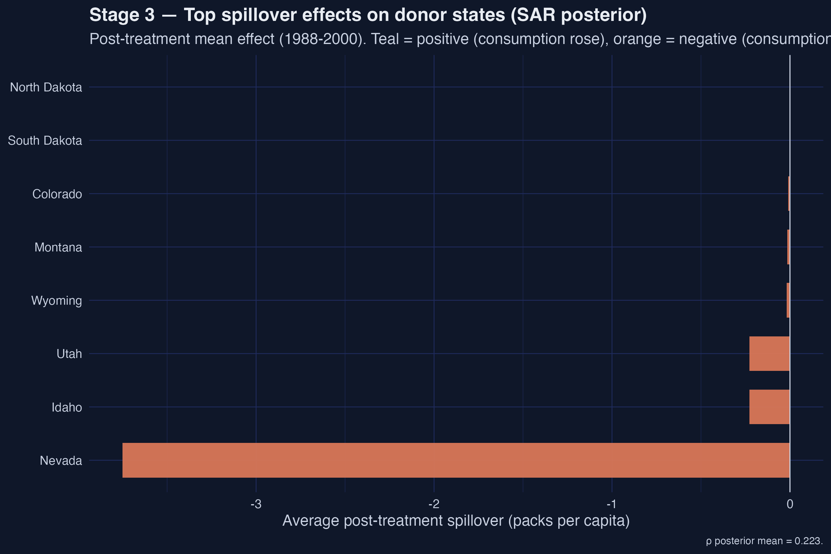
Almost the entire spillover lands on one state: Nevada

Top-8 donor states by absolute post-1988 spillover — Nevada’s −3.75 dwarfs every other state.

Nevada absorbs −3.75 packs/capita — 16× the next state (Idaho, −0.228) and more than 2,900× the smallest non-zero spillover (North Dakota). Nevada is California’s eastern neighbour, the only donor with a substantial contiguity link, so the row-normalized W concentrates the spillover mass there. This is the empirical signature of SUTVA failure.

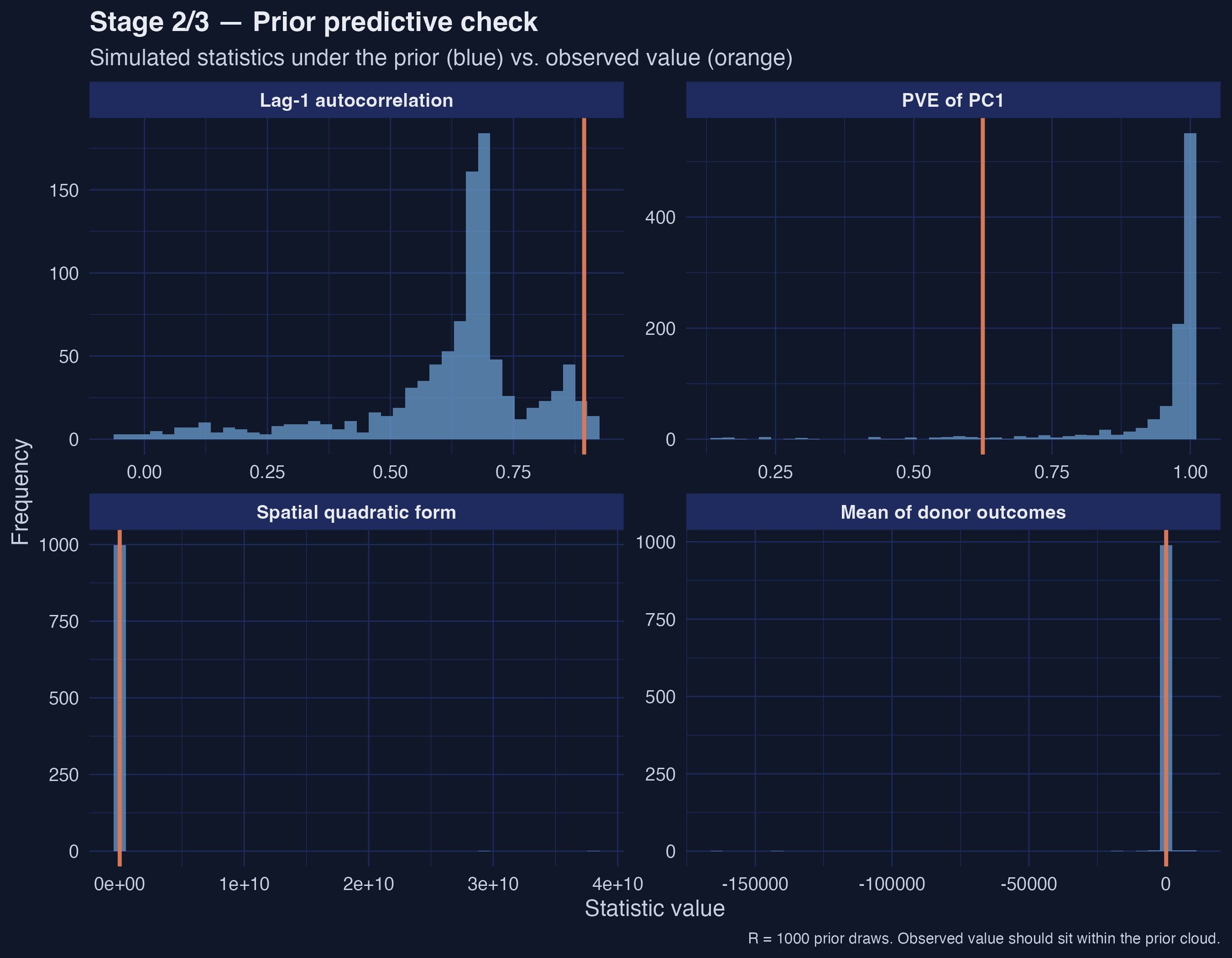
Before trusting the posterior, the prior must be compatible with the data

Prior predictive check on four summary statistics — all four observed orange lines land inside the simulated prior cloud, not in its tails.

1,000 joint prior draws are forward-simulated and compared to the observed donor panel on the mean, the spatial quadratic form y’Wy, lag-1 autocorrelation, and PC1 variance share. All four observed values land inside the cloud — the prior informs, it does not overwhelm. Had they landed in the tails, the posterior would be prior-driven.

The Resolution

Act III

All three estimators agree on sign and scale: Prop 99 worked

Stage	ATT	95% Interval	Active donors
Classical SCM	−18.46	[−22.21, −14.45]	4
Bayesian HS	−15.84	[−21.76, −9.48]	23
Bayesian Spatial SAR	−16.59	[−16.78, −16.39]	27

The headline ATT is robust; the donor pool’s shape is not — and the Stage-3 interval is artificially narrow (ESS(ρ) = 3 at tutorial scale).

Three reads. The sign and order of magnitude agree across all three — none of the intervals reaches zero. The active-donor count rises 4 → 23 → 27 as priors relax, so the sparse four-donor synthetic is one of many plausible counterfactuals. The Stage-3 CrI is the narrowest but least trustworthy because rho has not mixed at 5,000 iterations.

Does the SAR layer make this causal? No — two assumptions still carry the weight

Objection. A spatial model and machine-selected controls can’t manufacture identification.

Response. Correct. The ATT is identified only under conditional independence given \(X\) and parallel trends. The horseshoe just selects controls flexibly; the SAR layer just tests SUTVA — and rejects it. We evaluate a method, not a naive causal claim.

Steelman, don’t strawman. Bayesian machinery disciplines selection and surfaces spillovers; it does not relax the core identifying assumptions. The contribution is showing that SUTVA is testable and, here, false — which widens the policy’s measured reach.

SUTVA is empirically false here — and that widens Prop 99’s true reach

−3.75

Nevada’s post-treatment spillover (packs/capita) · 16× the next donor · direct evidence SUTVA is violated

The policy takeaway: reporting only California’s −18 understates Prop 99. The tax reshaped consumption on both sides of the California–Nevada border. When a treated unit has one or two highly-exposed neighbours, the classical “donors are unaffected” assumption can be tested — and here it fails decisively.

Let the data, not the simplex, choose your donors — and let the map tell you who else was treated.

The single takeaway. The headline effect is robust to every prior structure, but the synthetic’s composition is not, and SUTVA is false: Prop 99’s reach crosses the Nevada border. Relax the simplex to see the uncertainty; add the spatial layer to see the spillover.