Augmented Synthetic Control for Multiple Countries

Validate on a known truth, then trust the euro question

+6.241recovered vs true +6.250

0.128mean error after augmentation

0.74Spearman vs Papaioannou (2021)

Carlos Mendez

Nagoya University (GSID)

June 11, 2026

The Tension

Act I

We never see the counterfactual — so how do we trust a country-level estimate?

Did joining the euro make a country more productive? We see only the world that happened — never the path it would have taken.

Synthetic control builds the missing twin from a weighted recipe of donor countries. But classic SCM works only when the pre-treatment match is nearly perfect — and across structurally different countries it rarely is. So when can we believe it?

The estimand throughout is the ATT per treated country: actual minus synthetic, after the policy. The whole tension is that this is a difference of two estimated paths, one of which is a counterfactual we can never observe. Classic SCM’s Achilles heel is a small, heterogeneous donor pool — exactly the cross-country setting.

The honest answer: prove the estimator on a known truth before you trust the data

• Part 1 — a simulated 25-country panel where the true effect is injected and known
• Part 2 — a qualitative replication of Papaioannou (2021) on the real euro area
• The bridge — the Augmented SCM adds a Ridge bias-correction that earns its keep only on hard cases

We never trust a number on real data that the same method could not first recover on simulated ground truth.

This is the deck’s spine: validate-then-trust. The simulated panel is the lab; the euro replication is the field. The augmentation (Ridge outcome model) is the safety net that sits quietly until the pre-treatment fit is poor.

Where we’re going

• Three augsynth entry points — one unit, many units, many outcomes
• Validate each on simulated data with a known ATT
• When augmentation rescues a sign error plain SCM cannot
• Inference that refuses to over-claim — and can disagree with itself
• The euro question: synthetic Germany and the pooled EMU effect

The Investigation

Act II

One pipeline, three doors: route the panel by its shape, not its difficulty

Count the treated units and outcomes

• one unit, one outcome → single_augsynth
• many units, staggered → multisynth
• one unit, many outcomes → augsynth_multiout

They all converge

• convex donor weights \(W\) — a recipe
• optional Ridge bias correction
• ATT read off as actual \(-\) synthetic
• then inference

Formula mini-language: outcome ~ treatment | covariates.

The post opens with a Mermaid flowchart; reveal.js does not bundle mermaid, so it is re-expressed here as a two-column routing slide. The key point is that routing is by shape — count treated units and outcomes — and all three then share the same SCM-plus-Ridge machinery and the same ATT definition.

The lab: 25 countries, 39 years, a known effect injected into five of them

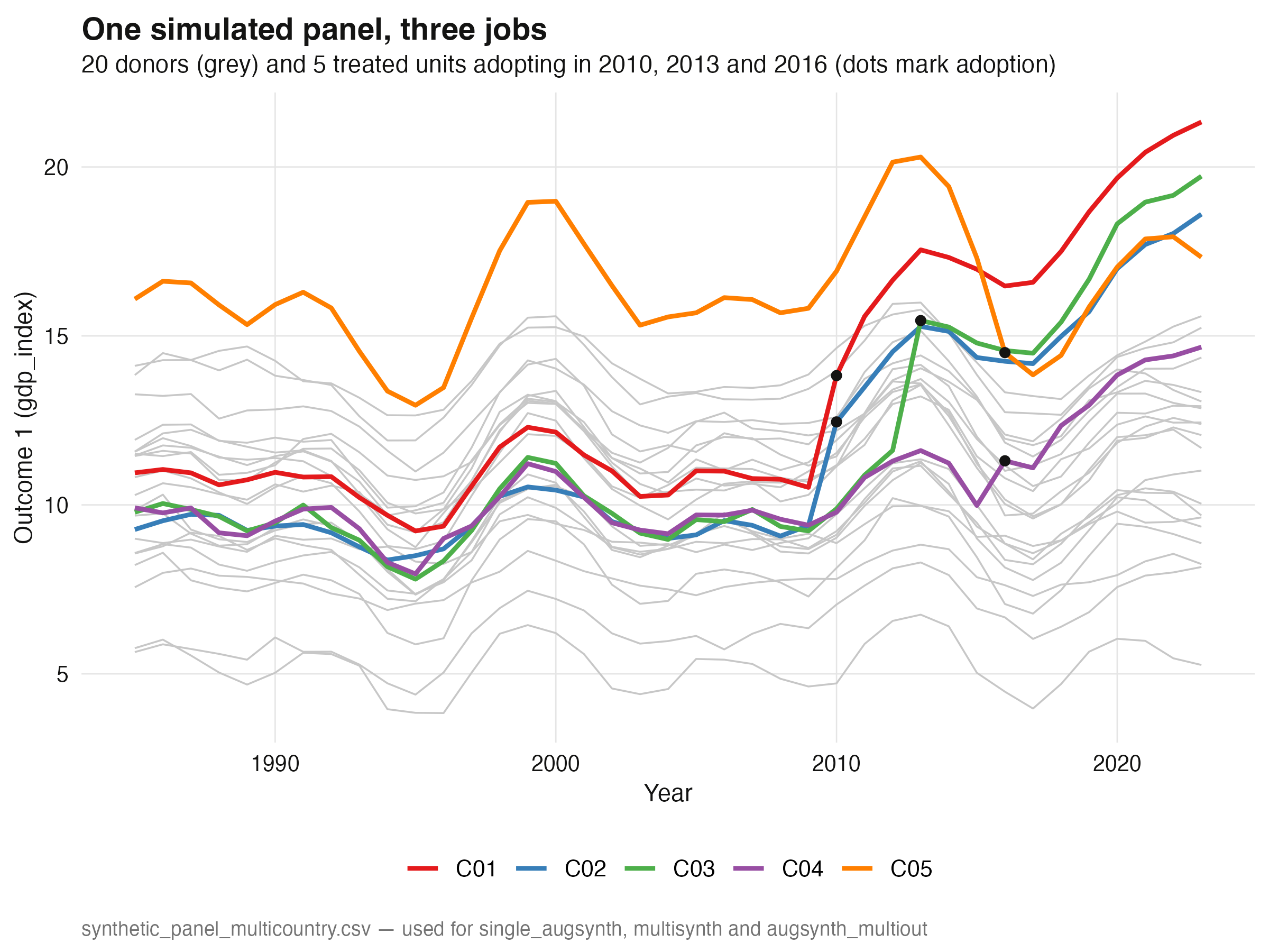
25 simulated paths — five treated units (colored) inside a cloud of 20 donors (grey); dots mark each adoption year.

975 rows: 25 units × 39 years (1985–2023). Five treated (C01–C05), 20 never-treated donors. The long pre-period is deliberate — it gives the inference procedures their power. C01–C04 are sparse convex blends of three donors each, so a clean synthetic exists; C05 is placed outside the donor hull on purpose to stress-test augmentation later. Treatment is staggered: 2010, 2010, 2013, 2016, 2016.

SCM solves a constrained recipe; ASCM subtracts what the fit still misses

\[W^{\star} = \arg\min_{W \in \Delta}\ \lVert X_1 - X_0 W \rVert_V \quad\text{s.t.}\quad w_j \ge 0,\ \sum_j w_j = 1\]

\[\hat\tau_t^{\,\mathrm{aug}} = \Big(Y_{1t} - \sum_j w_j Y_{jt}\Big) - \Big(\hat m_t(X_1) - \sum_j w_j\,\hat m_t(X_j)\Big)\]

The first term is the plain SCM gap; the second is the Ridge correction \(\hat m_t\). Perfect pre-fit → correction vanishes → ASCM \(=\) SCM.

W lives on the simplex Δ — non-negative weights summing to one, so the synthetic interpolates donors and never extrapolates. The augmented estimator is doubly robust: it is the SCM gap minus what the prognostic model m-hat (a Ridge regression on lagged outcomes) predicts the residual imbalance to be. When the donors already reproduce m-hat(X1), the correction is zero. This is why augmentation is insurance, not a free lunch.

single_augsynth recovers C01’s ATT to within 0.1% — and it’s significant

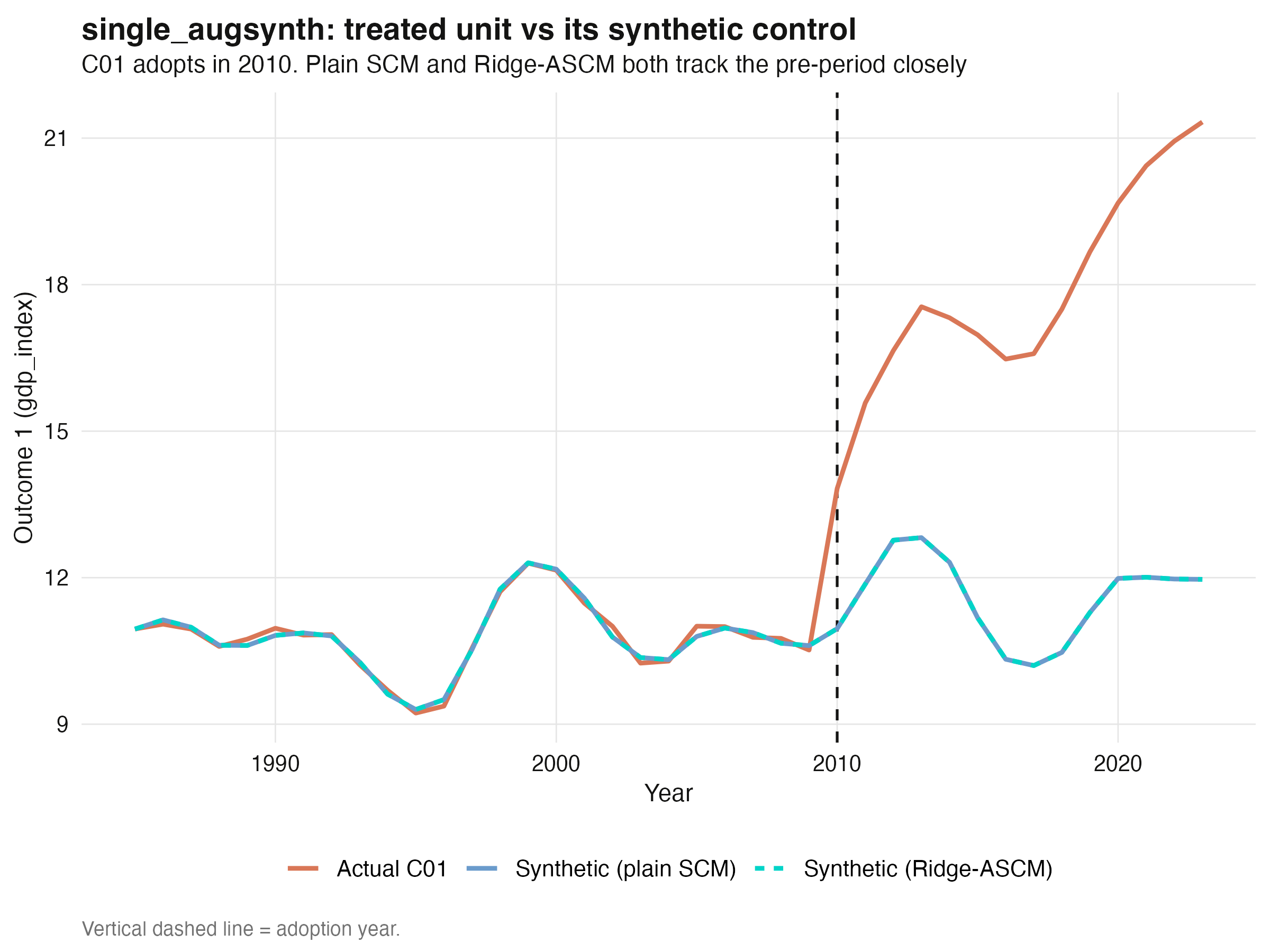
C01 actual vs its synthetic control: the synthetic tracks the pre-2010 path closely, then the gap opens.

True average post ATT for C01 is +6.250; plain SCM and Ridge-ASCM both return +6.241 — an error of 0.009. Jackknife+ 95% CI [5.998, 6.506] excludes zero; conformal p < 0.001. The two estimators agree because C01 sits inside the donor hull (scaled L2 = 0.135) and the Ridge λ ≈ 2639 all but switches augmentation off — the “when fit is good, ASCM ≈ SCM” lesson.

The dynamic gap lands on the true injected effect after treatment

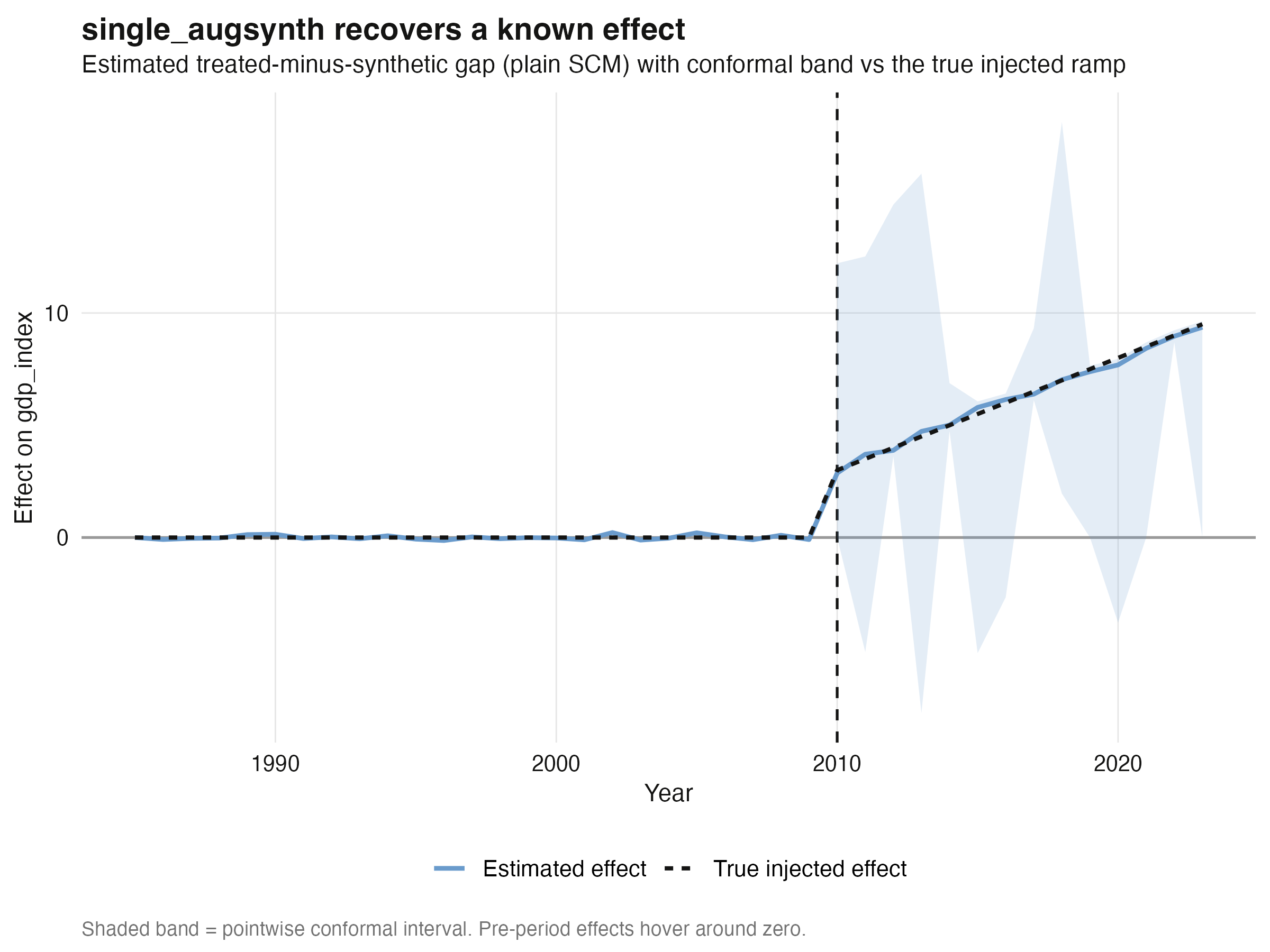
Estimated treated-minus-synthetic gap with its conformal band, overlaid on the true injected effect — near-perfect recovery.

The conformal band is pointwise over time. Pre-2010 the gap hovers at zero — the visual signature of a trustworthy synthetic control — and post-2010 it climbs right onto the dashed truth line. The conformal test is powerful precisely because the pre-period is long relative to the post-period, which is why this panel starts in 1985.

Six lines fit a single-unit ASCM in R

sim_single <- panel |>
  mutate(trt = as.integer(country == "C01" & year >= 2010))

sc_plain <- augsynth(gdp_index ~ trt, country, year, sim_single,
                     t_int = 2010, progfunc = "None",  scm = TRUE)
sc_ridge <- augsynth(gdp_index ~ trt, country, year, sim_single,
                     t_int = 2010, progfunc = "ridge", scm = TRUE)
summary(sc_plain, inf_type = "jackknife+")$average_att

The top-level augsynth() dispatches to single_augsynth() when it sees one treated unit and one intervention time. progfunc = “None” is plain SCM (Abadie’s classic estimator); progfunc = “ridge” turns on the bias-correction outcome model. Inference is requested at summary() time, not at fit time.

multisynth recovers the pooled ATT — and every per-unit sign, including a negative one

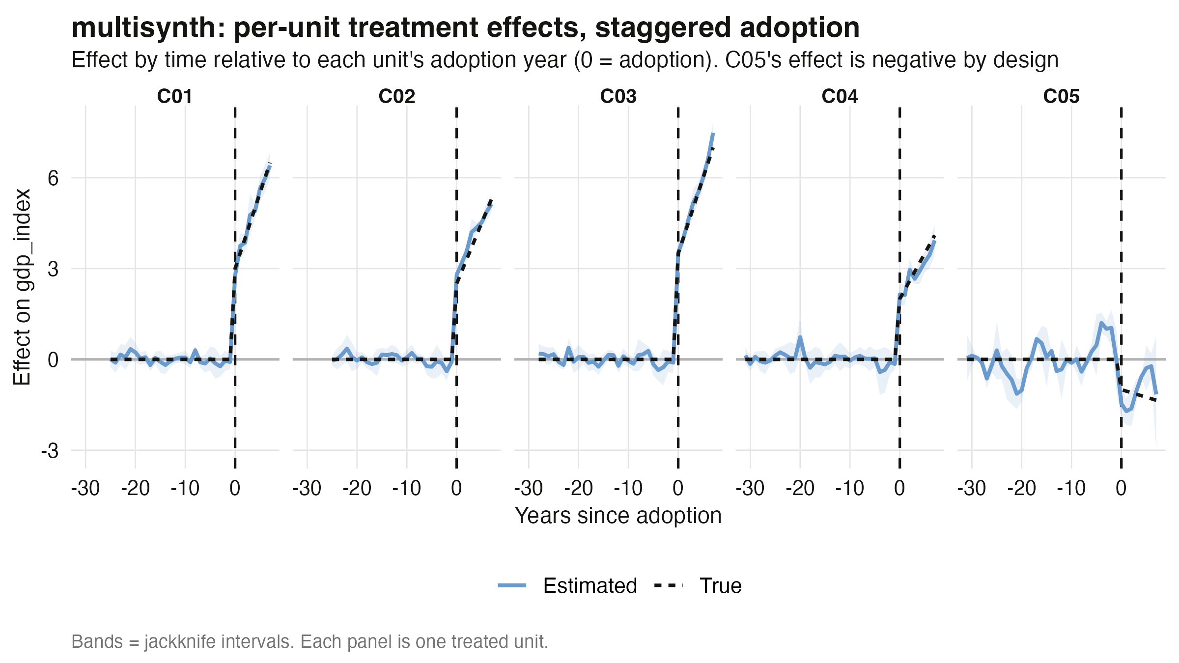
Per-unit treatment effects under staggered adoption: each unit’s estimate climbs to meet its dashed truth line — and C05 drops the opposite way.

multisynth needs no t_int — it infers each unit’s adoption from the 0→1 switch — and returns a pooled average plus per-unit effects, partially pooling them (auto nu = 0.583, global scaled L2 = 0.052). Pooled estimate 3.222 vs true 3.155. Every per-unit estimate has the right sign and ballpark, including C05’s negative −1.012 vs true −1.175. Per-unit values look smaller than single_augsynth’s 6.241 because multisynth averages over a common 8-lead window.

Same estimate, different verdict: jackknife says significant, the bootstrap says not

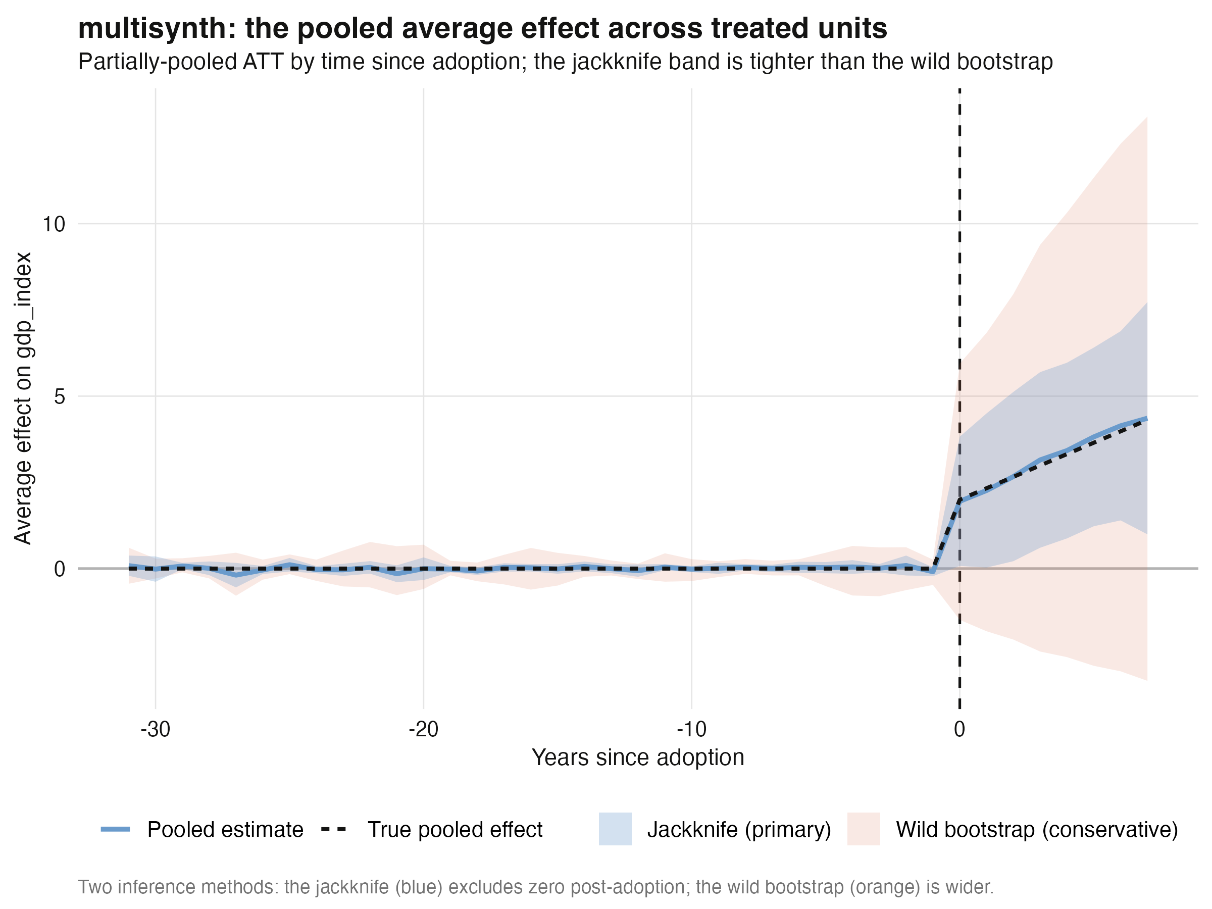
Pooled average effect with the tight jackknife band (excludes zero) and the wide wild-bootstrap band (includes zero), vs the true pooled effect.

This is the first concrete case of inference changing the headline. Pooled jackknife 95% CI [0.689, 5.754] excludes zero — significant. The wild bootstrap [−2.468, 9.779] is roughly 5× wider and includes zero — not significant. Neither is wrong: the jackknife asks “is the average across these units nonzero?”, the bootstrap additionally propagates how hard each counterfactual was to build. When they disagree, say so.

When a unit sits outside the donor hull, plain SCM gets the sign wrong

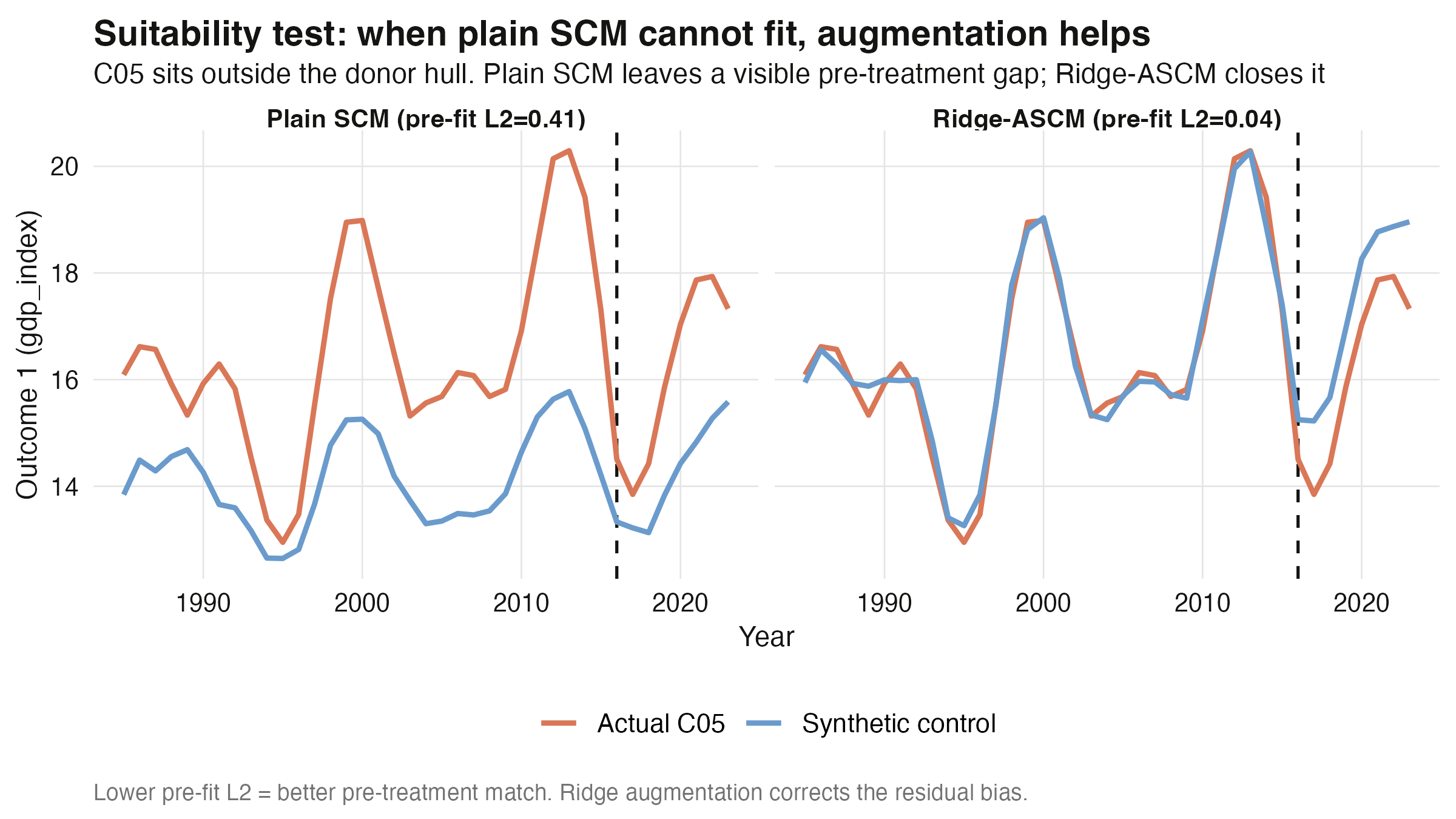
Suitability test for C05: plain SCM (blue) drifts from actual C05 (orange) before treatment; Ridge-ASCM pins them together pre-2016.

C05 was built outside the donor hull on purpose. No convex blend of donors reproduces its pre-period, so plain SCM estimates +1.896 when the truth is −1.175 — a sign error. Crucially its jackknife+ CI [−2.614, 6.407] includes zero and conformal p = 0.866, so honest inference correctly flags it as null: wrong AND not significant. Ridge-ASCM closes the pre-fit gap (scaled L2 0.414 → 0.036) and recovers −1.145.

Augmentation cuts the mean recovery error from 0.737 to 0.128

0.128

mean recovery error across five units after Ridge-ASCM — down from 0.737 under plain SCM

For the four well-fit units (C01–C04) plain SCM and Ridge-ASCM agree to the second decimal — augmentation does nothing. It earns its keep exactly once, on C05, the hard case. The practical rule: always read the pre-treatment scaled L2 imbalance; if it is small either method is fine, if it is large trust the augmented estimate and be suspicious of any synthetic control whose pre-period does not track.

The Resolution

Act III

On real data, synthetic Germany’s TFP runs +0.133 above its counterfactual after 1999

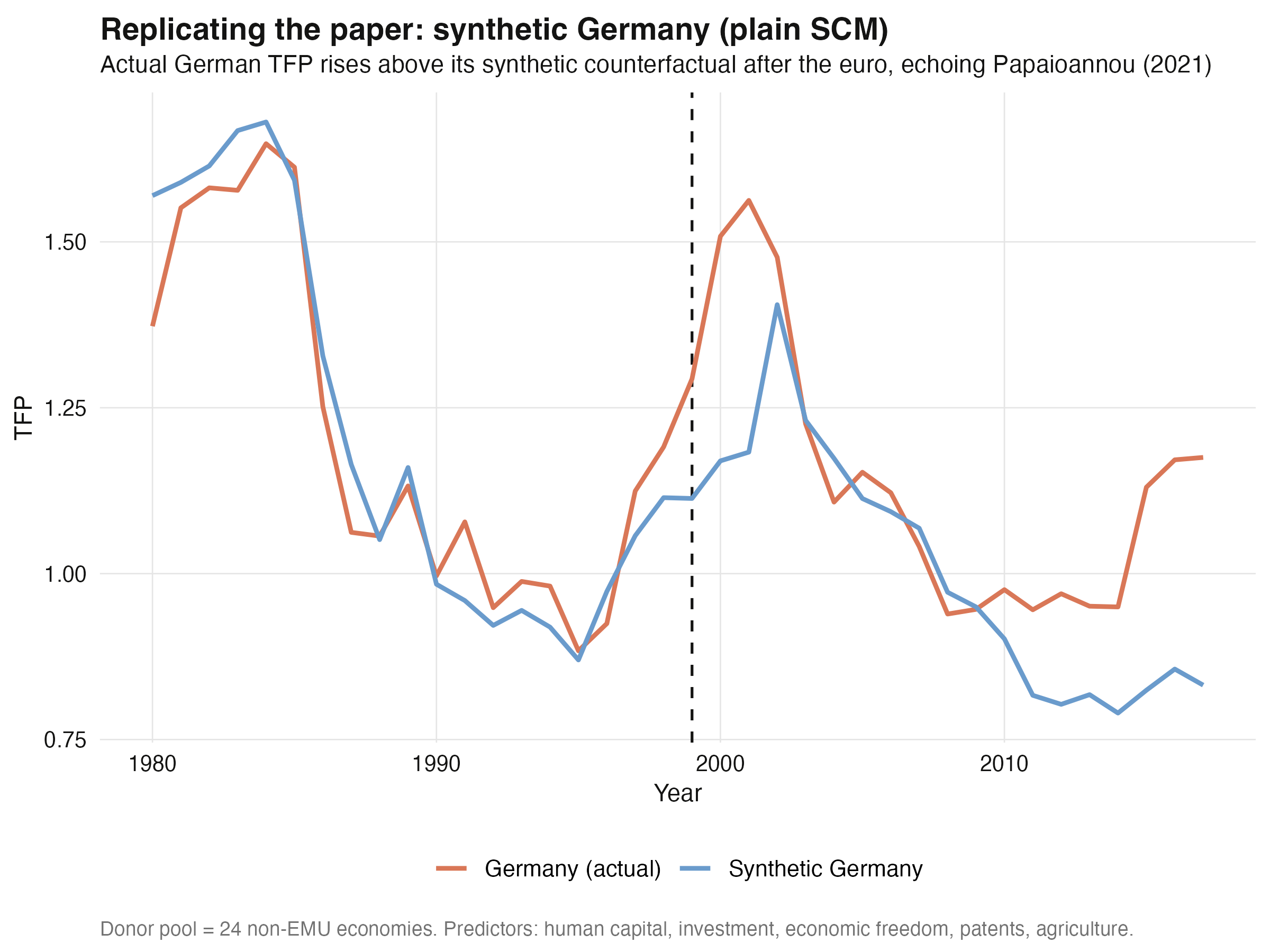
Synthetic Germany under plain SCM: actual TFP (orange) rises above the synthetic counterfactual (blue) after the 1999 euro launch.

Germany is fit against 24 non-euro donors, matching on pre-1999 TFP plus the paper’s predictors (human capital, investment share, economic freedom, patents, agriculture). Average ATT +0.133 TFP units — about +8.0% over 2000–07 and +19.3% over 2008–17. Pre-fit is good (scaled L2 = 0.30), so Ridge barely moves it (+0.127). Inference is honestly borderline: conformal p = 0.027 (significant) but jackknife+ [−0.082, 0.336] just includes zero. We flag it rather than pick the convenient answer.

The pooled euro average is a forgettable −0.016 — but the path tells the story

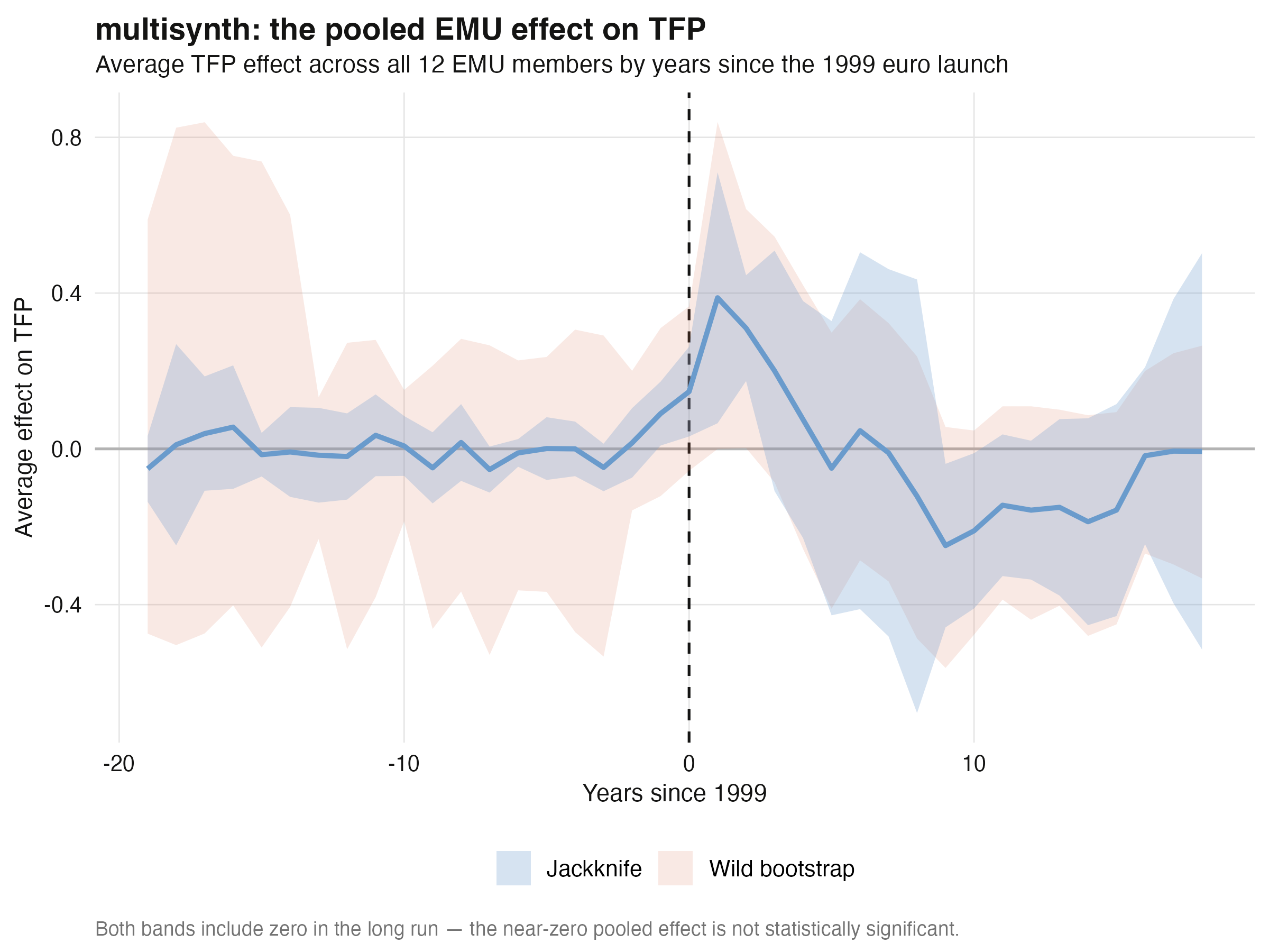
Pooled euro-area effect on TFP: flat pre-1999, a +0.39 early bump, eroded into negative territory by the 2008–2014 crisis, recovering by 2017.

multisynth across all 12 members is a simultaneous block design (all adopt in 1999). Pooled average ATT −0.016, jackknife [−0.282, 0.250] and bootstrap [−0.259, 0.231] both include zero — not significant under either. But the single number is misleading: the path is flat in the pre-period (no pre-trend, validating the design), rises to ≈ +0.39 in the early euro years, then slides negative through the crisis. Early gains and crisis losses cancel in the long-run average — exactly the arc Papaioannou describes.

Per-member fits reveal the heterogeneity the average hides

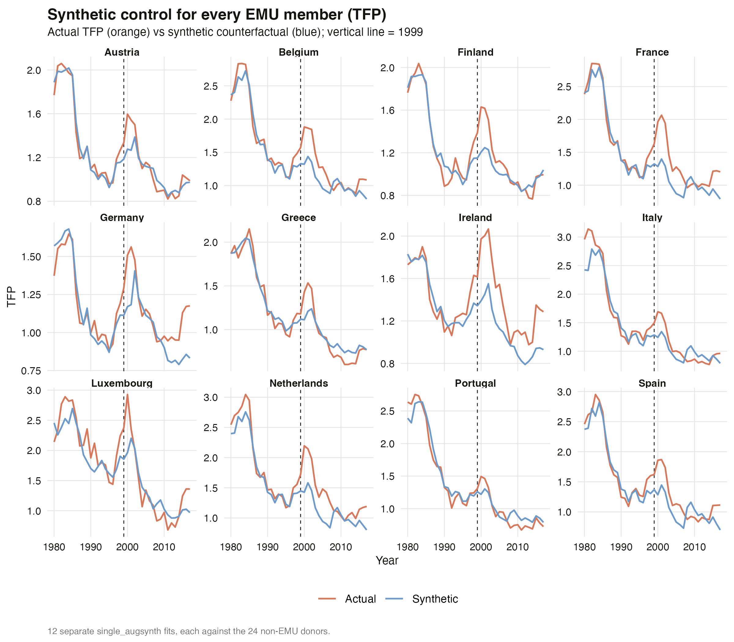
Synthetic control for every euro member: most run above their synthetic counterfactual after 1999; Greece and Portugal fall below post-crisis.

Twelve single_augsynth fits, each member vs the 24 donors. Most members run above their synthetic counterfactuals after 1999. Greece and Portugal converge to or fall below theirs after the crisis (Greece −12.4% in 2008–17, Portugal −14.3%) — matching the paper’s negative post-crisis contributions. Averages hide dynamics; the per-unit spread is the honest multi-country report.

ASCM ranks the euro winners just as Papaioannou did: Spearman 0.74

0.74

Spearman rank correlation between our ASCM TFP % effects and the paper’s, 2000–07 (Pearson 0.76)

Strong agreement given augsynth uses a different estimator and donor-matching scheme than the paper’s classic SCM. France (42.7% vs 43.6%) and the Netherlands (44.0% vs 38.2%) land almost on the 45-degree line; a few diverge in magnitude (Germany, Ireland) but not in sign. The pattern replicates: large euro-era gains for France, the Netherlands, Belgium, Spain, Ireland, and post-crisis reversals for Greece and Portugal. Qualitative replication — same signs, same ranking, same dynamic story — is the right bar for a method comparison.

The numbers line up around the 45-degree line, not on top of it

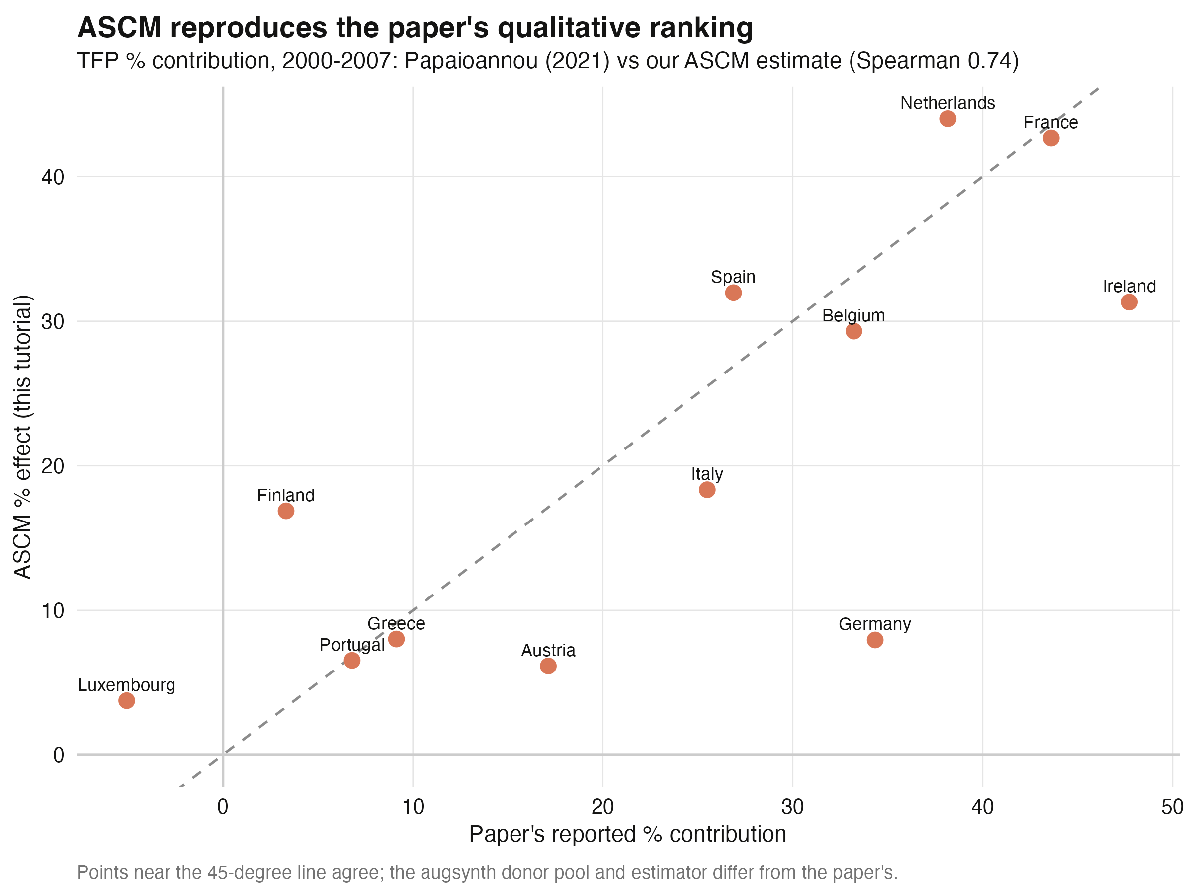
ASCM vs Papaioannou (2021): per-member TFP % contributions cluster around the 45-degree line, Spearman 0.74.

We do not reproduce the paper’s numbers exactly — and should not. Same signs, same ranking, same dynamic story is the right bar.

The estimators differ, so exact matches are not expected. All 12 members are positive in 2000–07. The scatter is the visual verdict: a method comparison passes when the qualitative pattern replicates, not when the decimals match.

Does ASCM make this causal? No — two assumptions still carry the weight

Objection. Machine-augmented donor weighting can’t manufacture identification — you’ve just dressed up a correlation.

Response. Correct, and we never claim otherwise. The ATT is identified only under no anticipation / a credible pre-treatment fit and the absence of confounding shocks coinciding with the euro. ASCM disciplines the counterfactual construction; it cannot rule out a contemporaneous shock. That is why we validated on simulated truth, read every pre-fit, and reported the borderline and null results as exactly that.

Steelman, don’t strawman. The robustness check (1992 vs 1999 dating: +0.138 vs +0.133) and the flat pre-trend address anticipation and pre-trend confounding, but they cannot exclude a coincident shock. Honest synthetic-control work disciplines selection and reports uncertainty; it does not relax the identifying assumptions.

Validate on a known truth, lean on augmentation only when the fit demands it, and read the path — not the average.

The single takeaway. Four habits make multi-country synthetic control honest: confirm the estimator recovers a known effect before trusting it on real data; read the pre-treatment imbalance every time and let augmentation work only on the hard cases; match the inference tool to the estimator and report when methods disagree; and read dynamics, because a near-zero average (−0.016) can hide a real +0.39 early bump erased by a crisis.