Spatial Dynamic Panel Data Modeling in R

Cigarette demand across 46 US states — where space meets habit

99.89%static SDM wins (Bayesian)

−1.23total static price elasticity

τ ≈ 0.86habit persistence dominates

Carlos Mendez

Nagoya University (GSID)

June 11, 2026

The Tension

Act I

When one state raises its cigarette tax, smokers cross the border

A tax hike in one state sends border-county smokers to a cheaper neighbour. So your consumption depends on your neighbours’ — a spatial spillover.

Standard panel methods assume each state stands alone. What do they miss?

This is the motivating story. Cross-border shopping makes the 46 states an interdependent system, not 46 isolated regressions. The whole deck is about what a model that ignores neighbours — and ignores yesterday — gets wrong.

A 30-year panel already whispers the answer: states stay where they start

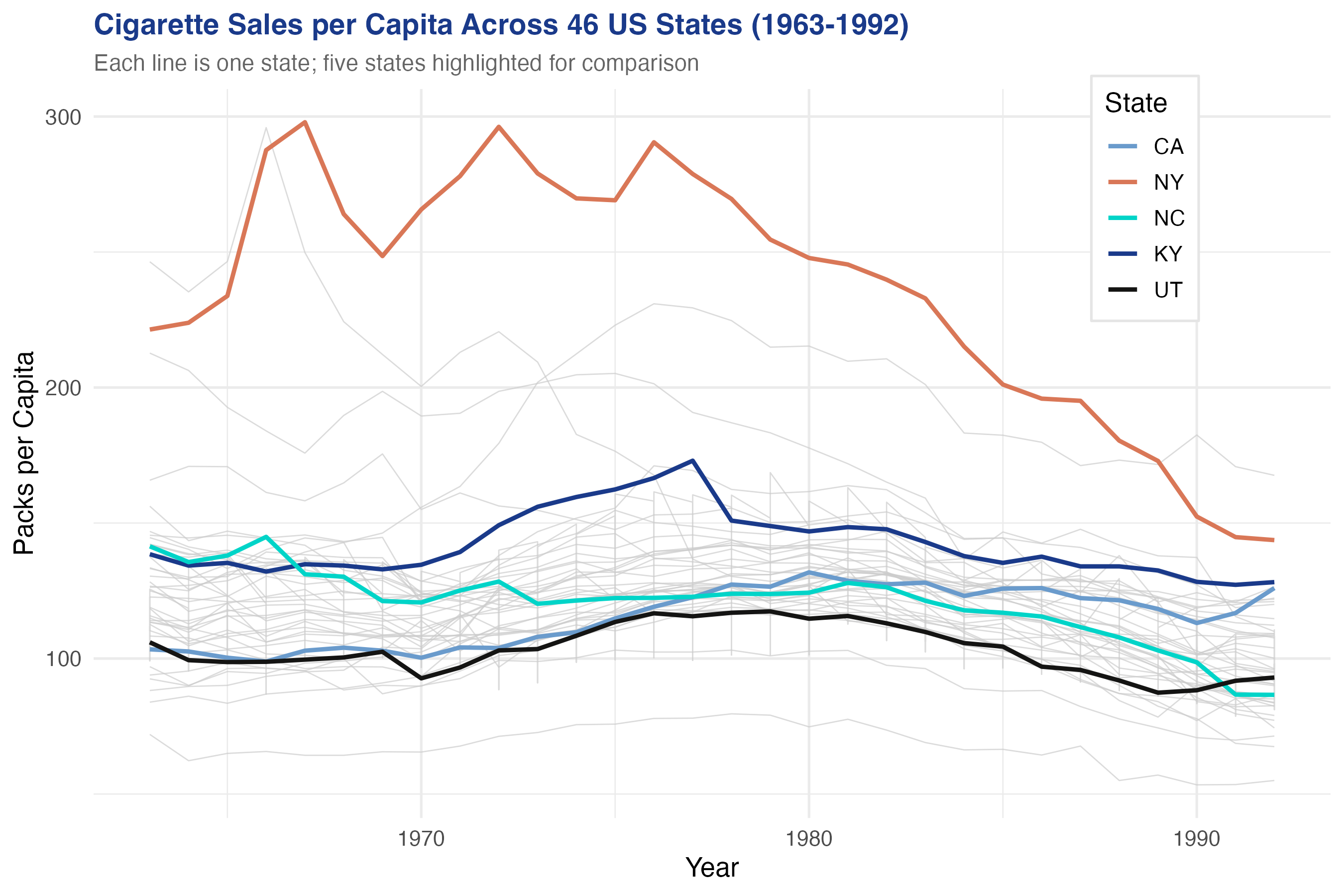
Cigarette sales per capita, 46 US states, 1963–1992. Five states highlighted. Heavy smokers stay heavy; a common downward trend after the late 1970s.

Spoiler figure for persistence. Kentucky (a tobacco state) stays above 150 packs per capita; Utah stays low. That visual stickiness foreshadows the dominant lagged-dependent-variable coefficient τ ≈ 0.86 in the dynamic models. The shared post-1970s decline is what time fixed effects will absorb.

Where we’re going

• The lab: a 46-state, 30-year panel and a contiguity matrix \(W\)
• Let the data choose the model — Bayesian comparison across six specifications
• Static SAR → SDM, with Lee-Yu bias correction
• Add time: dynamic SDM, habit persistence, and direct/indirect effects
• The lesson: ignore spillovers or habit, and tobacco-tax conclusions mislead

The Investigation

Act II

The lab: 46 states × 30 years of log-elasticities, neighbours from a \(W\) matrix

• Outcome — \(\log\) cigarette packs per capita (logc), 1,380 balanced observations
• Treatment-of-interest — \(\log\) real price (logp); also \(\log\) real income (logy)
• Neighbours — the usa46 binary contiguity matrix, row-normalized

Log-log: every coefficient is an elasticity — % change in consumption per % change in price.

State and year fixed effects absorb tobacco culture and national anti-smoking trends. The Cigar dataset (Baltagi 1992). pimin — minimum neighbour price — is left out on purpose: its correlation with the spatial lag W·logp is 0.92, so the SDM’s W·logp term captures the same cross-border channel more flexibly.

Neighbours are sparse: 188 of 2,116 pairs, ~4 neighbours per state

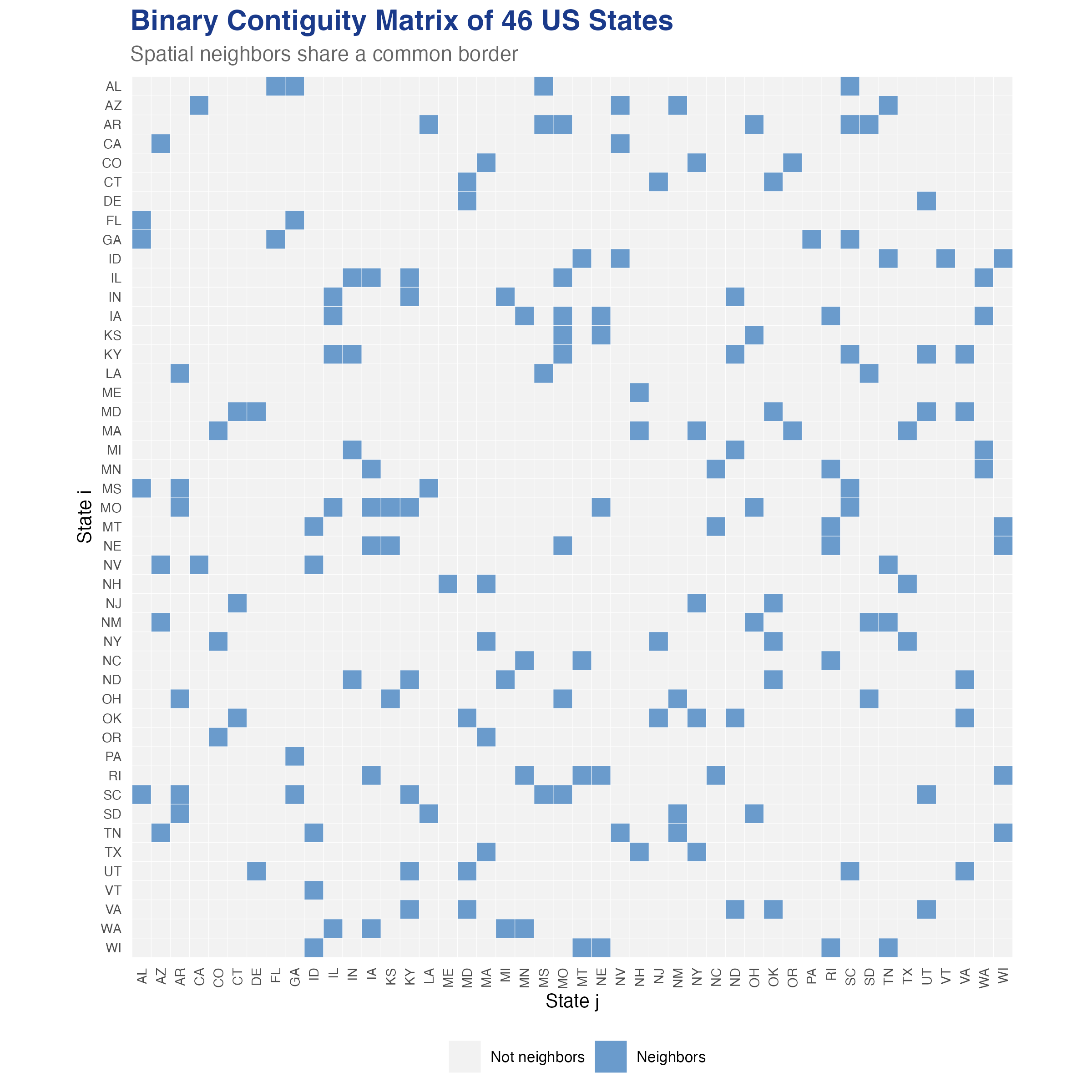
Binary contiguity matrix of 46 US states. Coloured cell = a shared border. Only 8.9% of cells are neighbours.

188 non-zero entries, 8.9% density, 4.09 neighbours on average. Maine has 1 neighbour; Missouri has 8. After row-normalization, the spatial lag Wy of any variable is the simple average across a state’s contiguous neighbours — so ρWy reads as “how much your neighbours’ average pulls you.”

Six spatial models, one equation — they differ in where space enters

\[y_t = \rho W y_t + X_t \beta + W X_t \theta + u_t, \quad u_t = \lambda W u_t + \epsilon_t\]

• \(\rho\) — neighbours’ outcomes spill over (SAR)
• \(\theta\) — neighbours’ covariates spill over (SLX)
• \(\lambda\) — spatial correlation in the errors (SEM)
• The SDM keeps \(\rho\) and \(\theta\); OLS sets all three to zero

blmpSDPD() scores every model at once with a log-marginal posterior — no ad-hoc sequence of Wald tests.

The general nesting structure: SDM is SAR plus spatial lags of X; SAR, SEM, SLX, SDEM are restrictions. Bayesian comparison assigns a probability to every candidate simultaneously, which is exactly what we want for a “which specification?” question.

Let the data choose: the static SDM wins with 99.89% posterior probability

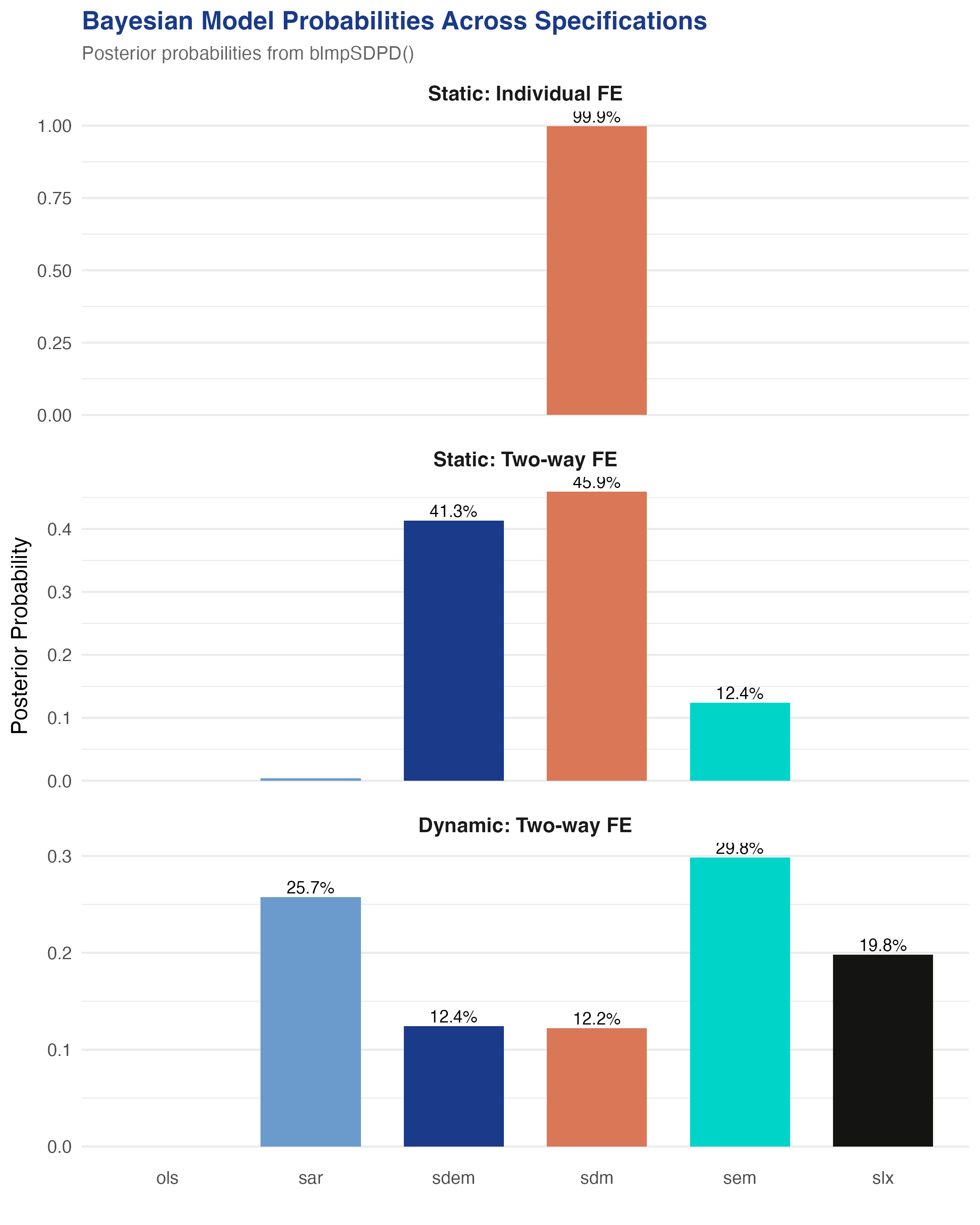
Posterior model probabilities across three specifications — static individual FE, static two-way FE, dynamic two-way FE.

Under individual FE the SDM gets 99.89%; SDEM 0.11%; everything else ≈ 0. OLS and SLX never win — spatial dependence is unambiguously present. Adding two-way FE tightens the race (SDM 45.9% vs SDEM 41.3%); adding dynamics flattens it entirely, foreshadowing that the lagged dependent variable absorbs the persistence spatial lags used to carry.

SDM dominates the static race — but dynamics flatten every model

Specification	Top model	Prob.	Runner-up	Prob.
Static, individual FE	SDM	99.89%	SDEM	0.11%
Static, two-way FE	SDM	45.92%	SDEM	41.31%
Dynamic, two-way FE	SEM	29.84%	SAR	25.73%

Once the lagged outcome enters, the spatial signal weakens — the data can no longer tell the spatial models apart.

Three takeaways: (1) spatial dependence is real (OLS/SLX never win); (2) SDM is the preferred static model — both ρWy and WXθ matter; (3) dynamics dissolve the discrimination, because yt−1 captures the temporal persistence the spatial lags were borrowing.

SAR makes neighbours’ consumption pull your own — ρ = 0.187, highly significant

\[y_t = \rho W y_t + X_t \beta + \mu_i + \gamma_t + \epsilon_t\]

• Two-way FE: \(\rho = 0.187\), \(t = 6.52\) — a state inherits a fraction of its neighbours’ consumption
• Price elasticity \(\beta_{\text{logp}} = -0.995\); income \(\beta_{\text{logy}} = 0.464\), both significant
• With individual FE only, \(\rho\) inflates to 0.298 and price collapses to \(-0.53\) — time trends confound it

The story of why two-way FE matters: dropping time effects lets common national trends masquerade as price effects (−0.53) and inflate the spatial coefficient (0.298). Once year effects are in, price snaps to ≈ −1.0 and income becomes significant — cigarettes are a normal good at the state level.

Six lines fit a spatial-Durbin panel with Lee-Yu correction in R

data("usa46", package = "SDPDmod")
W <- rownor(usa46)                       # row-normalize the contiguity matrix
mod <- SDPDm(logc ~ logp + logy, data = data1, W = W,
             index = c("state","year"), model = "sdm",
             effect = "twoways", LYtrans = TRUE)   # Lee-Yu bias correction
summary(impactsSDPDm(mod))               # direct / indirect / total

SDPDm() is the maximum-likelihood workhorse: model = “sdm” adds WXθ to SAR; LYtrans = TRUE applies the Lee-Yu transformation; impactsSDPDm() turns the raw coefficients into direct, indirect, and total effects. The whole pipeline — Bayesian selection, estimation, decomposition — lives in one package.

Lee-Yu corrects the small-sample bias, lifting ρ from 0.223 to 0.262

The 46 + 30 = 76 fixed effects create an incidental-parameter bias in spatial ML.

• Uncorrected SDM: \(\rho = 0.223\) → Lee-Yu: \(\rho = 0.262\) (a 17% upward correction)
• Slopes barely move (\(\beta_{\text{logp}}\): \(-1.003 \to -1.001\)) — expected with \(T = 30\)

For short panels (\(T < 10\)) the correction would matter far more; here it mainly rescues \(\rho\).

Lee-Yu (2010) transforms the data to concentrate the fixed effects out before estimation. The uncorrected estimator understates spatial dependence. With 30 time periods the slope bias is small, but ρ — the parameter most sensitive to the incidental-parameter problem — moves a meaningful 17%. We adopt the Lee-Yu version as the preferred static SDM.

SDM adds neighbours’ covariates — and flips the income spillover negative

Effect	logp \(\hat\beta\)	logy \(\hat\beta\)
Direct	−1.010	0.588
Indirect (spillover)	−0.219	−0.197
Total	−1.230	0.391

The income spillover is negative (−0.20): richer neighbours pull your consumption down — a channel the SAR cannot see.

Price tells the familiar story: direct −1.01, indirect −0.22, total −1.23. But income reverses sign relative to SAR (+0.10 there): the significant W·logy ≈ −0.31 means richer neighbours reduce own-state demand, plausibly through substitution toward premium or out-of-state channels. The SDM’s WXθ terms are what make this visible.

Ignore spillovers and you understate the price response by 22%

−1.23

Total static-SDM price elasticity vs a \(-1.01\) direct effect — spillovers add 22%

This is the headline of the static analysis. A state evaluating a tax increase with a non-spatial model (β ≈ −1.0) underestimates the true consumption reduction once neighbour feedback is counted. Spatial spillovers are economically meaningful: ~18% of the total effect.

Cigarettes are habit-forming — so yesterday belongs in the model

\[y_t = \rho W y_t + \tau y_{t-1} + \eta W y_{t-1} + X_t \beta + W X_t \theta + \mu_i + \gamma_t + \epsilon_t\]

• \(\tau y_{t-1}\) — own past consumption (habit persistence)
• \(\eta W y_{t-1}\) — neighbours’ past consumption (spatiotemporal diffusion)

A static \(\rho\) must absorb both spatial spillover and serial correlation — so it is biased upward.

Nicotine addiction makes last year’s smokers this year’s smokers. If the model omits yt−1, the contemporaneous spatial coefficient has to do double duty, conflating “your neighbours smoke” with “you smoked last year, and so did they.” Adding the temporal lag separates the two.

Add time and the spatial story shrinks: τ = 0.86 dominates, ρ falls to 0.16

Parameter	Static SDM (LY)	Dynamic SDM (LY)
\(\tau\) (logc\(_{t-1}\))	—	0.864
\(\rho\) (W·logc)	0.262	0.162
\(\beta_{\text{logp}}\)	−1.001	−0.271
W·logp	0.091 (n.s.)	0.196 (sig.)

Habit persistence is the dominant force; the static SDM was overstating contemporaneous spatial dependence.

τ = 0.864 (t = 67) is by far the largest, most precise parameter — about 87% of last year’s consumption carries over. ρ falls from 0.262 to 0.162 once we control for that persistence: much of what looked spatial was temporal. And W·logp turns positive and significant — the next slide.

The dynamic SDM uncovers cross-border shopping: W·logp = +0.20, significant

When a neighbour raises its price, your consumption rises — smokers buy more in your now-cheaper state.

• Static SDM: \(W\cdot\text{logp} = 0.091\), not significant — masked by \(\rho W y\)
• Dynamic SDM: \(W\cdot\text{logp} = 0.196\), \(t = 4.46\) — the cross-border signal emerges

The spatial lag of consumption hid the effect; only proper dynamics reveal it.

This is the substantive payoff. The static model’s ρWy term soaks up the cross-border channel, so W·logp looks null. Once yt−1 and Wyt−1 are in, the price-of-neighbours coefficient stands free and positive — exactly the cross-border shopping the opening story predicted.

Short-run vs long-run: a 1% price hike cuts demand 0.26% now, 1.93% eventually

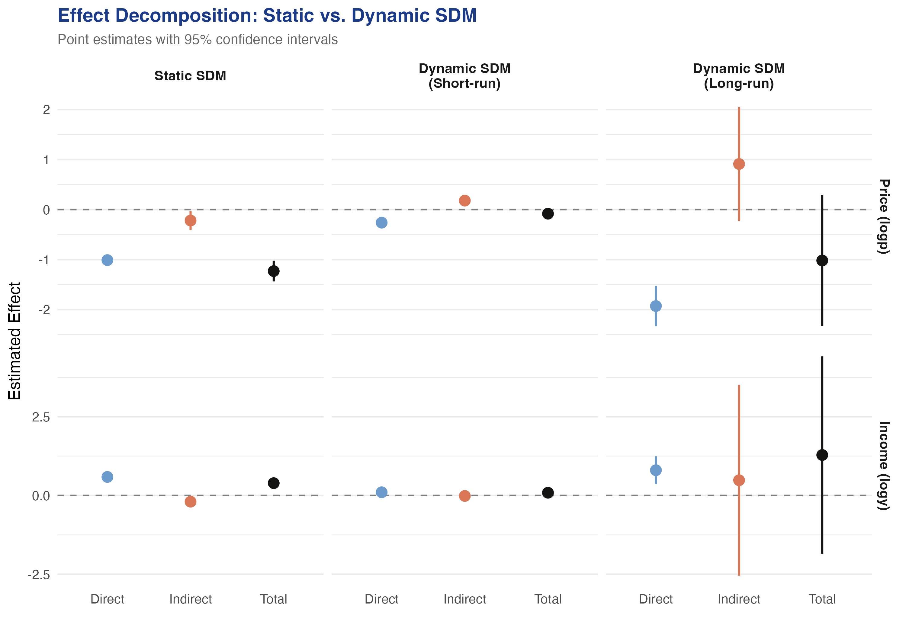
Direct, indirect, and total effects of price and income — static SDM vs dynamic SDM short-run and long-run.

Habit persistence (τ = 0.864) amplifies the initial shock: short-run direct price elasticity −0.26 balloons to −1.93 in the long run, a ~7× snowball. The static SDM (−1.01 direct) overstates the immediate response by ~4×. Short-run indirect price is positive (+0.18) — cross-border shopping again — partly offsetting the direct effect; long-run totals carry wide standard errors, so steady-state predictions need caution.

The Resolution

Act III

Habit persistence rules: τ ≈ 0.86 dwarfs the spatial coefficient

0.864

Temporal-lag coefficient \(\tau\) in the dynamic SDM (\(t = 67\)) — vs a contemporaneous \(\rho = 0.16\)

The most precisely estimated parameter in the entire analysis. ~87% of consumption carries over year to year. Space matters — ρ = 0.16 is significant — but it is small next to the inertia of addiction. Static models that omit τ mistake persistence for spillover.

Does any of this estimate a causal tax effect? Not without the usual assumptions

Objection. The W·logp coefficient and the impacts read like causal cross-border effects — but the data are observational.

Response. Correct — this is a modeling workflow, not an identified policy experiment.

• FE strip time-invariant state heterogeneity and common shocks
• A causal tax elasticity still needs no time-varying confounders
• And a stable spatial process (\(|\tau + \rho\eta| < 1\))

Steelman, don’t strawman. Two-way fixed effects strip state heterogeneity and common shocks, and the spatial/dynamic terms model interdependence — but that is not identification. The post is careful: SDPDmod gives a principled way to model spatial and temporal dependence, but it does not manufacture identification. The elasticities are descriptive of an interdependent system under FE; reading them as the causal effect of a tax requires the standard panel assumptions plus stationarity of the dynamic-spatial system.

One dataset, three lessons the workflow makes visible

• Spillovers are real — total static price elasticity \(-1.23\) is 22% above the direct \(-1.01\)
• Habit dominates dynamics — \(\tau \approx 0.86\); short-run price response is a quarter of the static estimate
• Cross-border shopping emerges — \(W\cdot\text{logp} = +0.20\), only once dynamics are specified

The summary slide. Each lesson maps to a section: Bayesian comparison + impacts (spillovers), dynamic SDM (habit), dynamic SDM W·logp (cross-border). Robustness: a 2nd-order W lifts ρ to 0.449 and makes W·logp significant — spillovers may reach beyond immediate neighbours.

Ignore your neighbours or ignore yesterday, and your tobacco-tax forecast is wrong.

The single takeaway, resolving the Act-I hook. Cross-border shopping (space) and addiction (time) jointly shape cigarette demand; a model that drops either one — the standard panel regression, or a static spatial model — gives a misleading answer for tax policy. SDPDmod lets you keep both.