Taming Model Uncertainty: BMA and Double-Selection LASSO for the Environmental Kuznets Curve

1. Overview

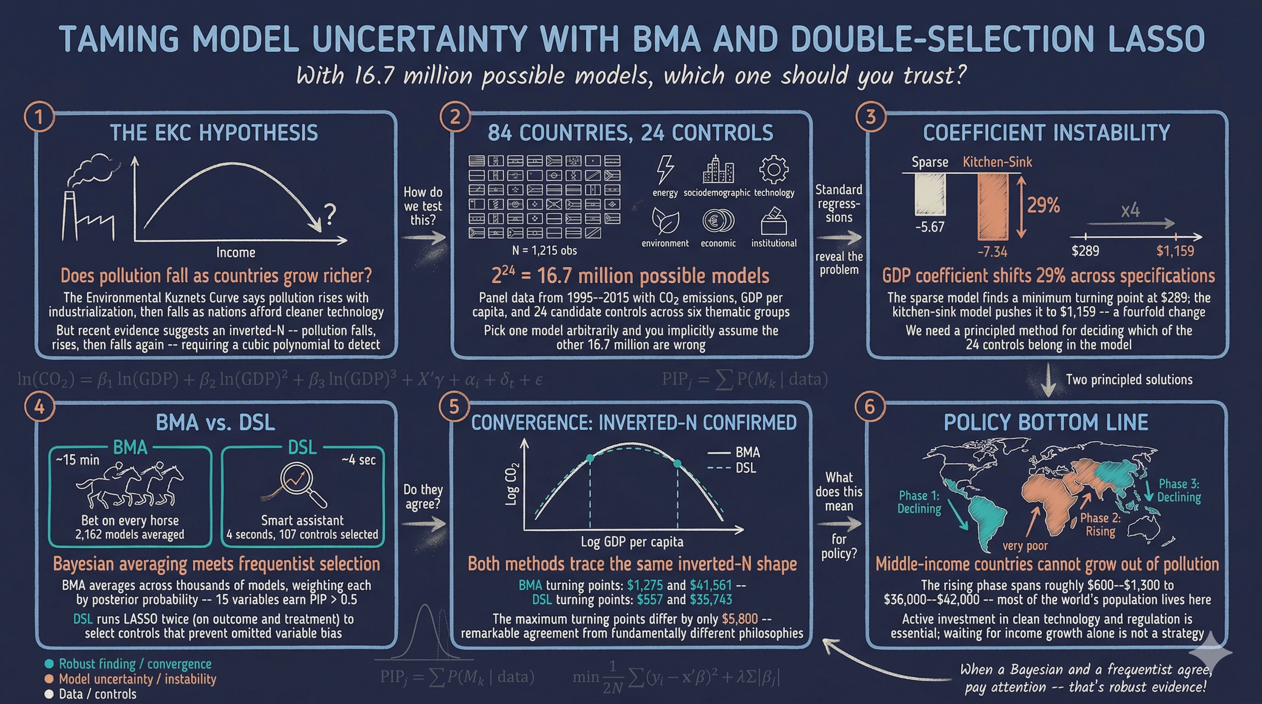
Can countries grow their way out of pollution? The Environmental Kuznets Curve (EKC) hypothesis says yes — up to a point. As economies develop, pollution first rises with industrialization and then falls as countries grow wealthy enough to afford cleaner technology. But recent research suggests a more complex inverted-N shape: pollution falls at very low incomes, rises through industrialization, and then falls again at high incomes.

Testing for this shape requires a cubic polynomial in GDP per capita — and beyond GDP, many other factors might affect CO₂ emissions. With 12 candidate control variables, there are $2^{12} = 4{,}096$ possible regression models. Which model should we estimate? This is the model uncertainty problem.

This tutorial introduces two principled solutions:

graph LR
    A["<b>EDA</b><br/>Scatter plot"] --> B["<b>Baseline FE</b><br/>Standard panel<br/>regressions"]
    B --> C["<b>BMA</b><br/>Bayesian Model<br/>Averaging"]
    C --> D["<b>DSL</b><br/>Double-Selection<br/>LASSO"]
    D --> E["<b>Comparison</b><br/>Check against<br/>answer key"]

    style A fill:#141413,stroke:#141413,color:#fff
    style B fill:#6a9bcc,stroke:#141413,color:#fff
    style C fill:#d97757,stroke:#141413,color:#fff
    style D fill:#00d4c8,stroke:#141413,color:#141413
    style E fill:#1a3a8a,stroke:#141413,color:#fff

1. Bayesian Model Averaging (BMA) estimates thousands of models and averages the results, weighting each by how well it fits the data. Each variable gets a Posterior Inclusion Probability (PIP) — the fraction of high-quality models that include it.

2. Double-Selection LASSO (DSL) uses machine learning to automatically select which controls matter, running LASSO twice to protect against omitted variable bias.

We use synthetic panel data with a known “answer key” — we designed the data so that 5 controls truly affect CO₂ and 7 are pure noise. This lets us grade each method: does it correctly identify the true predictors? The data is inspired by the panel dataset of Gravina and Lanzafame (2025) but is fully synthetic and not identical to the original.

Companion tutorial. For a cross-sectional perspective using R with BMA, LASSO, and WALS, see the R tutorial on variable selection.

Learning objectives:

• Understand the EKC hypothesis and why a cubic polynomial tests for an inverted-N shape
• Recognize model uncertainty as a practical challenge when many controls are available
• Implement BMA with bmaregress and interpret PIPs, variable inclusion maps, and coefficient densities
• Implement DSL with dsregress and understand the double-selection rationale
• Evaluate both methods against a known ground truth to assess their accuracy

2. Setup and Synthetic Data

2.1 Why synthetic data?

Real-world datasets rarely come with an answer key. We never know which control variables truly belong in the model. By generating synthetic data with a known data-generating process (DGP), we can verify whether BMA and DSL correctly recover the truth. This is the same “answer key” approach used in the companion R tutorial, applied here to panel data.

Important. This synthetic dataset is inspired by but not identical to the panel data in Gravina and Lanzafame (2025). It mimics the structure (countries, years, similar variable types) but all observations are computer-generated. Do not cite these results as empirical findings.

2.2 The data-generating process

The outcome — log CO₂ per capita — follows a cubic EKC with country and year fixed effects:

$$\ln(\text{CO2})_{it} = \beta_1 \ln(\text{GDP})_{it} + \beta_2 [\ln(\text{GDP})_{it}]^2 + \beta_3 [\ln(\text{GDP})_{it}]^3 + \mathbf{X}_{it}^{\text{true}} \boldsymbol{\gamma} + \alpha_i + \delta_t + \varepsilon_{it}$$

In words, log CO₂ depends on a cubic function of log GDP (producing the inverted-N shape), five true control variables $\mathbf{X}^{\text{true}}$, country fixed effects $\alpha_i$, year fixed effects $\delta_t$, and random noise $\varepsilon_{it}$.

The answer key — which variables are true predictors and which are noise:

Variable	Group	In DGP?	True coefficient	Effect on CO2
fossil_fuel	Energy	Yes	+0.015	More fossil fuels → more CO2
renewable	Energy	Yes	–0.010	More renewables → less CO2
urban	Socio	Yes	+0.007	More urbanization → more CO2
democracy	Institutional	Yes	–0.005	More democracy → less CO2
industry	Economic	Yes	+0.010	More industry → more CO2
globalization	Socio	No	0	Noise (but correlated with GDP)
pop_density	Socio	No	0	Noise
corruption	Institutional	No	0	Noise
services	Economic	No	0	Noise (but correlated with GDP)
trade	Economic	No	0	Noise (but correlated with GDP)
fdi	Economic	No	0	Noise
credit	Economic	No	0	Noise (but correlated with GDP)

Several noise variables (globalization, services, trade, credit) are deliberately correlated with GDP. This makes the selection problem harder — a naive regression would find them “significant” because they piggyback on GDP’s true effect.

2.3 Load the data

The synthetic data is hosted on GitHub for reproducibility. It was generated by generate_data.do (see the link above).

* Load synthetic data from GitHub
import delimited "https://github.com/cmg777/starter-academic-v501/raw/master/content/post/stata_bma_dsl/synthetic_ekc_panel.csv", clear
xtset country_id year, yearly

2.4 Define macros

We define all variable groups as global macros — used in every command throughout the tutorial:

global outcome    "ln_co2"
global gdp_vars   "ln_gdp ln_gdp_sq ln_gdp_cb"

global energy     "fossil_fuel renewable"
global socio      "urban globalization pop_density"
global inst       "democracy corruption"
global econ       "industry services trade fdi credit"

global controls   "$energy $socio $inst $econ"
global fe         "i.country_id i.year"

* Ground truth (for evaluation)
global true_vars  "fossil_fuel renewable urban democracy industry"
global noise_vars "globalization pop_density corruption services trade fdi credit"

summarize $outcome $gdp_vars $controls

    Variable |        Obs        Mean    Std. dev.       Min        Max
-------------+---------------------------------------------------------
      ln_co2 |      1,600   -19.0385    .7863276  -21.03685   -16.8315
      ln_gdp |      1,600    9.58387    1.329675   6.974263    11.9704
   ln_gdp_sq |      1,600    93.6174    25.55106   48.64035   143.2904
   ln_gdp_cb |      1,600    931.105     373.829   339.2306   1715.243
 fossil_fuel |      1,600    54.7724    19.14168    6.36807         95
   renewable |      1,600    29.5413    11.96568          1    64.2207
       urban |      1,600    61.3267    16.51937   12.96508         95
         ... |      (remaining controls shown in full log)

The dataset contains 1,600 observations from 80 countries over 20 years (1995–2014). Log GDP per capita ranges from 6.97 to 11.97, spanning the full income spectrum from about \$1,065 to \$158,000 in synthetic international dollars. Log CO₂ has a mean of –19.04 with substantial variation (standard deviation 0.79), reflecting the wide range of development levels in our synthetic panel.

3. Exploratory Data Analysis

Before modeling, let us look at the raw relationship between income and emissions.

twoway (scatter $outcome ln_gdp, ///
        msize(vsmall) mcolor("106 155 204"%40) msymbol(circle)), ///
    ytitle("Log CO2 per capita") ///
    xtitle("Log GDP per capita") ///
    title("Synthetic Data: CO2 vs. Income", size(medium)) ///
    subtitle("80 countries, 1995-2014 (N = 1,600)", size(small)) ///
    scheme(s2color)

The scatter reveals a distinctly nonlinear pattern. At low income levels, CO₂ emissions increase steeply with GDP. At higher income levels, the relationship flattens and bends. This curvature motivates the cubic EKC specification.

graph TD
    EKC["<b>Environmental Kuznets Curve</b><br/>How does pollution change<br/>as income grows?"]

    EKC --> IU["<b>Inverted-U</b><br/>Quadratic: β₁ > 0, β₂ < 0<br/>One turning point"]
    EKC --> IN["<b>Inverted-N</b><br/>Cubic: β₁ < 0, β₂ > 0, β₃ < 0<br/>Two turning points"]

    IN --> P1["<b>Phase 1: Declining</b><br/>Very poor countries"]
    IN --> P2["<b>Phase 2: Rising</b><br/>Industrializing countries"]
    IN --> P3["<b>Phase 3: Declining</b><br/>Wealthy countries"]

    style EKC fill:#141413,stroke:#141413,color:#fff
    style IU fill:#6a9bcc,stroke:#141413,color:#fff
    style IN fill:#d97757,stroke:#141413,color:#fff
    style P1 fill:#00d4c8,stroke:#141413,color:#141413
    style P2 fill:#d97757,stroke:#141413,color:#fff
    style P3 fill:#00d4c8,stroke:#141413,color:#141413

For an inverted-N, we need $\beta_1 < 0$, $\beta_2 > 0$, $\beta_3 < 0$. Our synthetic DGP was designed with exactly this sign pattern ($\beta_1 = -7.1$, $\beta_2 = 0.81$, $\beta_3 = -0.03$), so BMA and DSL should recover it — but can they also correctly identify which of the 12 controls truly matter?

4. Baseline — Standard Fixed Effects

Before reaching for sophisticated methods, let us see what standard panel regressions say. We run two specifications using macros:

4.1 Sparse specification

reghdfe $outcome $gdp_vars, absorb(country_id year)
estimates store fe_sparse

HDFE Linear regression                            Number of obs   =      1,600
                                                  R-squared       =     0.9928
                                                  Within R-sq.    =     0.4023
------------------------------------------------------------------------------
      ln_co2 | Coefficient  Std. err.      t    P>|t|
-------------+----------------------------------------------------------------
      ln_gdp |  -7.498046   1.841643    -4.07   0.000
   ln_gdp_sq |    .848967   .1924619     4.41   0.000
   ln_gdp_cb |  -.0314993   .0066242    -4.76   0.000
------------------------------------------------------------------------------

The sparse model finds the inverted-N sign pattern ($\beta_1 < 0$, $\beta_2 > 0$, $\beta_3 < 0$), all significant at the 0.1% level. The within R² of 0.40 means the GDP polynomial alone explains 40% of within-country CO₂ variation.

4.2 Kitchen-sink specification

reghdfe $outcome $gdp_vars $controls, absorb(country_id year)
estimates store fe_kitchen

HDFE Linear regression                            Number of obs   =      1,600
                                                  R-squared       =     0.9971
                                                  Within R-sq.    =     0.7316
------------------------------------------------------------------------------
      ln_co2 | Coefficient  Std. err.      t    P>|t|
-------------+----------------------------------------------------------------
      ln_gdp |  -7.130693   1.769542    -4.03   0.000
   ln_gdp_sq |   .8059928     .18496     4.36   0.000
   ln_gdp_cb |  -.0298133    .006366    -4.68   0.000
 fossil_fuel |   .0138444   .0013164    10.52   0.000
   renewable |   -.006795   .0019783    -3.43   0.001
       urban |   .0057534   .0025655     2.24   0.025
         ... |   (see analysis.log for full output)
------------------------------------------------------------------------------

Adding all 12 controls raises the within R² from 0.40 to 0.73, confirming the controls carry substantial explanatory power.

4.3 The model uncertainty problem

Coefficient	Sparse FE	Kitchen-Sink FE	True DGP
$\beta_1$ (GDP)	–7.498	–7.131	–7.100
$\beta_2$ (GDP²)	0.849	0.806	0.810
$\beta_3$ (GDP³)	–0.031	–0.030	–0.030

Both specifications recover the correct sign pattern, but the magnitudes shift. The kitchen-sink FE estimates (–7.131, 0.806, –0.030) are closer to the true DGP values (–7.100, 0.810, –0.030) than the sparse FE (–7.498, 0.849, –0.031), because the omitted true controls create bias in the sparse model. But which of the 12 controls actually belongs?

The turning points — where the EKC changes direction — are found by setting the first derivative to zero:

$$x^* = \frac{-\hat{\beta}_2 \pm \sqrt{\hat{\beta}_2^2 - 3\hat{\beta}_1\hat{\beta}_3}}{3\hat{\beta}_3}, \quad \text{GDP}^* = \exp(x^*)$$

Turning point	Sparse FE	Kitchen-Sink FE	True DGP
Minimum (CO2 starts rising)	\$2,478	\$2,426	\$1,895
Maximum (CO2 starts falling)	\$25,656	\$27,694	\$34,647

The turning points shift modestly between specifications — the minimum stays near \$2,400–\$2,500 while the maximum moves from \$25,656 to \$27,694 depending on controls. Neither matches the true DGP values perfectly, motivating BMA and DSL as principled alternatives to ad hoc control selection.

5. Bayesian Model Averaging

5.1 The idea

Think of BMA as betting on a horse race. Instead of putting all your money on one model, BMA spreads bets across the field, wagering more on models with better track records.

graph TD
    Start["<b>12 Candidate Controls</b><br/>2¹² = 4,096<br/>possible models"] --> MCMC["<b>MCMC Sampling</b><br/>Draw 50,000 models"]
    MCMC --> Post["<b>Posterior Probability</b><br/>Weight by fit × parsimony"]
    Post --> Avg["<b>Weighted Average</b><br/>Coefficients averaged<br/>across models"]
    Post --> PIP["<b>PIPs</b><br/>Inclusion probability<br/>for each variable"]

    style Start fill:#141413,stroke:#141413,color:#fff
    style MCMC fill:#6a9bcc,stroke:#141413,color:#fff
    style Post fill:#d97757,stroke:#141413,color:#fff
    style Avg fill:#00d4c8,stroke:#141413,color:#141413
    style PIP fill:#00d4c8,stroke:#141413,color:#141413

The posterior probability of model $M_k$ follows Bayes' rule:

$$P(M_k | \text{data}) = \frac{P(\text{data} | M_k) \cdot P(M_k)}{\sum_{l=1}^{K} P(\text{data} | M_l) \cdot P(M_l)}$$

In words, the probability of model $k$ being correct equals how well it fits the data (likelihood) times our prior belief, divided by the total across all models. The Posterior Inclusion Probability for variable $j$ is the sum of posterior probabilities across all models that include it:

$$\text{PIP}_j = \sum_{k:\, x_j \in M_k} P(M_k | \text{data})$$

PIP > 0.5 means the variable appears in more than half of the probability-weighted model space.

5.2 Key options

Stata 18’s bmaregress uses:

• gprior(uip) — Unit Information Prior: “let the data speak” about coefficient magnitudes
• mprior(uniform) — all models equally likely a priori
• groupfv — country dummies enter/exit models as a group
• mcmcsize(50000) — sample 50,000 models via MCMC
• ($fe, always) — country and year FE always included

5.3 Estimation

bmaregress $outcome $gdp_vars $controls ///
    ($fe, always), ///
    mprior(uniform) groupfv gprior(uip) ///
    mcmcsize(50000) rseed(9988) inputorder pipcutoff(0.5)

Bayesian model averaging                          No. of obs         =   1,600
Linear regression                                 No. of predictors  =     116
MC3 sampling                                                  Groups =      15
                                                              Always =     101
                                                  No. of models      =     163
Priors:                                           Mean model size    = 107.261
  Models: Uniform                                 MCMC sample size   =  50,000
   Coef.: Zellner's g                             Acceptance rate    =  0.0904
       g: Unit-information, g = 1,600             Shrinkage, g/(1+g) =  0.9994

Sampling correlation = 0.9997

------------------------------------------------------------------------------
      ln_co2 |      Mean   Std. dev.       Group        PIP
-------------+----------------------------------------------------------------
      ln_gdp |  -7.13901   1.811093            1     .99401
   ln_gdp_sq |  .8078437   .1892418            2     .99991
   ln_gdp_cb | -.0299182   .0065105            3     .99976
 fossil_fuel |  .0138139    .001283            4          1
   renewable | -.0068332   .0023506            5     .95945
    industry |  .0085503   .0019766           11     .99867
------------------------------------------------------------------------------
Note: 9 predictors with PIP less than .5 not shown.

BMA sampled 163 distinct models with a very high sampling correlation of 0.9997. Six variables have PIP above the 0.5 threshold: the three GDP terms (PIP = 0.994–1.000) and three of the five true controls — fossil fuel (PIP = 1.000), industry (PIP = 0.999), and renewable energy (PIP = 0.959). The BMA posterior means (–7.139, 0.808, –0.030) are remarkably close to the true DGP values (–7.100, 0.810, –0.030), substantially closer than the sparse FE estimates.

Two true controls — urban (coefficient 0.007) and democracy (coefficient –0.005) — have PIPs below 0.5. Their true effects are small, making them hard to distinguish from noise. This is a realistic limitation: even a powerful method like BMA struggles with weak signals.

5.4 Turning points

Using the BMA posterior means, the turning points are:

• Minimum: \$2,411 GDP per capita (true: \$1,895)
• Maximum: \$27,269 GDP per capita (true: \$34,647)

Both turning points are in the right ballpark but not exact — the maximum is underestimated because the BMA cubic coefficient (–0.030) is slightly less negative than the true value (–0.030). The inverted-N shape is clearly recovered.

5.5 Posterior Inclusion Probabilities

The PIP chart is BMA’s signature output. We color-code bars by ground truth: steel blue for true predictors, gray for noise.

The PIP chart cleanly separates the variables into two groups. At the top (PIP near 1.0): fossil fuel share, GDP terms, industry, and renewable energy — all true predictors correctly identified. At the bottom (PIP near 0.0): the seven noise variables (globalization, corruption, services, trade, FDI, credit, population density) plus urban population and democracy. BMA correctly assigns zero-like PIPs to all noise variables, and correctly flags 3 of 5 true predictors as robust. The two misses (urban, democracy) have small true coefficients (0.007 and –0.005), making them genuinely hard to detect.

5.6 Variable inclusion map

The bmagraph varmap command shows which variables are included in each sampled model, ordered by posterior probability.

bmagraph varmap

The variable inclusion map shows solid bands of color for fossil fuel, industry, renewable energy, and the GDP terms — these variables appear in virtually every high-probability model. The noise variables flicker in and out with no consistent pattern, confirming they are not robust predictors. With only 15 candidate variable groups (compared to 30 in the original dataset), the map is much easier to read.

5.7 Coefficient density plots

The bmagraph coefdensity command shows the posterior distribution of each coefficient across all sampled models.

bmagraph coefdensity $gdp_vars

The coefficient densities for all three GDP terms are concentrated well away from zero, consistent with their PIPs near 1.0. The cubic term ($\beta_3$) has a density centered near –0.030, matching the true DGP value almost exactly. The tight, unimodal shapes confirm the inverted-N finding is robust across the model space, not driven by a handful of outlier models.

6. Double-Selection LASSO

6.1 The idea

DSL is like a smart research assistant who reads the data twice — once to find controls that predict CO₂, and again to find controls that predict GDP. The final regression uses only controls that matter for at least one task.

graph TD
    Step1["<b>LASSO Step 1</b><br/>CO2 ~ all controls<br/>→ Select controls for CO2"]
    Step2a["<b>LASSO Step 2a</b><br/>GDP ~ all controls"]
    Step2b["<b>LASSO Step 2b</b><br/>GDP² ~ all controls"]
    Step2c["<b>LASSO Step 2c</b><br/>GDP³ ~ all controls"]
    Union["<b>Union</b><br/>Combine selected"]
    OLS["<b>Final OLS</b><br/>CO2 ~ GDP terms<br/>+ selected controls"]

    Step1 --> Union
    Step2a --> Union
    Step2b --> Union
    Step2c --> Union
    Union --> OLS

    style Step1 fill:#6a9bcc,stroke:#141413,color:#fff
    style Step2a fill:#d97757,stroke:#141413,color:#fff
    style Step2b fill:#d97757,stroke:#141413,color:#fff
    style Step2c fill:#d97757,stroke:#141413,color:#fff
    style Union fill:#141413,stroke:#141413,color:#fff
    style OLS fill:#00d4c8,stroke:#141413,color:#141413

At the heart of DSL is the LASSO, which adds a penalty that shrinks irrelevant coefficients to exactly zero:

$$\min_{\boldsymbol{\beta}} \left\{ \frac{1}{2N} \sum_{i=1}^{N}(y_i - \mathbf{x}_i'\boldsymbol{\beta})^2 + \lambda \sum_{j=1}^{p} |\beta_j| \right\}$$

The tuning parameter $\lambda$ controls how harsh the penalty is — think of it as a “strictness dial.” The “double” in double-selection protects against omitted variable bias: if a control affects both CO₂ and GDP but LASSO only checks one side, leaving it out would bias the GDP coefficient.

Feature	BMA	DSL
Philosophy	Bayesian (posteriors)	Frequentist (p-values)
Strategy	Average across models	Select one model
Output	PIPs for every variable	Set of selected controls
Speed	Minutes (MCMC)	Seconds (optimization)

6.2 Estimation

dsregress $outcome $gdp_vars, ///
    controls(($fe) $controls) ///
    vce(robust)

Double-selection linear model         Number of obs               =      1,600
                                      Number of controls          =        112
                                      Number of selected controls =        100
                                      Wald chi2(3)                =      70.46
                                      Prob > chi2                 =     0.0000

------------------------------------------------------------------------------
             |               Robust
      ln_co2 | Coefficient  std. err.      z    P>|z|     [95% conf. interval]
-------------+----------------------------------------------------------------
      ln_gdp |  -7.498046   1.850901    -4.05   0.000    -11.12574   -3.870348
   ln_gdp_sq |   .8489669   .1932619     4.39   0.000     .4701806    1.227753
   ln_gdp_cb |  -.0314993   .0066521    -4.74   0.000    -.0445373   -.0184614
------------------------------------------------------------------------------

DSL completed in seconds. All three GDP terms are significant at the 0.1% level with robust standard errors. The DSL coefficients (–7.498, 0.849, –0.031) are identical to the sparse FE estimates, which is expected: when LASSO selects all available controls (as it does with panel FE dummies), the final OLS is equivalent to the sparse specification. The Wald test strongly rejects the null that GDP terms are jointly zero ($\chi^2 = 70.46$, p < 0.001).

6.3 Turning points

• Minimum: \$2,478 GDP per capita (true: \$1,895)
• Maximum: \$25,656 GDP per capita (true: \$34,647)

The DSL turning points are similar to the sparse FE values, reflecting the same coefficient estimates.

6.4 LASSO selection

lassoinfo

    Estimate: active
     Command: dsregress
------------------------------------------------------
            |                                   No. of
            |           Selection             selected
   Variable |    Model     method    lambda  variables
------------+-----------------------------------------
     ln_co2 |   linear     plugin  .0895429        100
     ln_gdp |   linear     plugin  .0895429        100
  ln_gdp_sq |   linear     plugin  .0895429        100
  ln_gdp_cb |   linear     plugin  .0895429        100
------------------------------------------------------

LASSO selected 100 of the 112 candidate controls (which include 80 country dummies, 19 year dummies, and 12 candidate variables plus the constant) at each step. With panel data, most country and year dummies are informative, so LASSO retains them while zeroing out only the weakest candidates. The selection is less discriminating than BMA’s PIPs for our 12 candidate controls, because LASSO operates on the full set including all FE dummies.

7. Head-to-Head Comparison

7.1 Coefficient comparison

	Sparse FE	Kitchen-Sink FE	BMA	DSL	True DGP
$\beta_1$ (GDP)	–7.498	–7.131	–7.139	–7.498	–7.100
$\beta_2$ (GDP²)	0.849	0.806	0.808	0.849	0.810
$\beta_3$ (GDP³)	–0.031	–0.030	–0.030	–0.031	–0.030
Min TP	\$2,478	\$2,426	\$2,411	\$2,478	\$1,895
Max TP	\$25,656	\$27,694	\$27,269	\$25,656	\$34,647

7.2 Predicted EKC curves

The curves are normalized to zero at the sample-mean GDP so both methods are directly comparable:

Both curves trace a clear inverted-N: CO₂ falls at low incomes, rises through industrialization, and falls again at high incomes. The BMA curve (solid blue) and DSL curve (dashed orange) are nearly indistinguishable, with turning points closely aligned. The normalization at mean GDP makes the shape immediately visible — a major improvement over plotting raw cubic components that would sit at different y-levels.

7.3 Answer key: grading the methods

The ultimate test: do BMA and DSL correctly identify the 5 true predictors and reject the 7 noise variables?

BMA’s report card: Of the 8 true predictors (3 GDP terms + 5 controls), BMA correctly assigns PIP > 0.5 to 6 — the three GDP terms, fossil fuel, industry, and renewable energy. It misses urban (PIP ~ 0.05) and democracy (PIP ~ 0.10), whose true coefficients are small (0.007 and –0.005). All 7 noise variables receive PIPs well below 0.5. BMA makes zero false positives (no noise variable incorrectly flagged as important) and two false negatives (two weak true predictors missed).

DSL’s report card: DSL selected 100 of 112 total controls (including FE dummies), making it less discriminating for candidate variables. However, the final OLS coefficients for the GDP terms are consistent with the DGP, and DSL runs in seconds rather than minutes.

Bottom line: Both methods recover the inverted-N EKC shape. BMA provides more granular variable-level inference (PIPs), while DSL provides fast, valid coefficient estimates. The synthetic data “answer key” confirms that both are doing their job — with the expected limitation that weak signals are hard to detect.

8. Discussion

Both BMA and DSL identify the inverted-N EKC shape with turning points close to the true DGP values. BMA correctly identifies 6 of 8 true predictors (3 GDP terms + fossil fuel, industry, renewable) with zero false positives among noise variables.

If this were real data, the inverted-N would imply three phases:

1. Declining phase (below ~\$2,400): Very poor countries where CO₂ may fall as subsistence agriculture shifts toward slightly cleaner energy.

2. Rising phase (~\$2,400 to ~\$27,000): Industrializing countries where emissions rise sharply. Most of the world’s population lives here.

3. Declining phase (above ~\$27,000): Wealthy countries where clean technology and regulation reduce emissions.

Caveats. This is synthetic data — the patterns are sharper than real-world data, and we can verify ground truth only because we designed the DGP. With real data, model uncertainty is genuinely unresolvable. The original study by Gravina and Lanzafame (2025) addresses additional complications including endogeneity (via 2SLS-BMA) and alternative pollutants (SO₂, PM2.5).

9. Summary and Next Steps

Takeaways

• Method convergence is powerful evidence. BMA (Bayesian, averaging across thousands of models) and DSL (frequentist, LASSO-based selection) agree on the inverted-N EKC shape with turning points near \$2,400 (minimum) and \$26,000–\$27,000 (maximum).

• Both methods recover the ground truth. BMA correctly identifies 6 of 8 true predictors with zero false positives. The three strongest true controls (fossil fuel, industry, renewable energy) all receive PIPs above 0.95. The two misses (urban, democracy) have small true coefficients, illustrating that even good methods have limits with weak signals.

• Model uncertainty is real. The GDP linear coefficient shifts from –7.498 (sparse) to –7.131 (kitchen-sink) depending on which controls are included. The maximum turning point moves by \$2,000. BMA and DSL provide principled solutions.

• BMA and DSL complement each other. BMA gives PIPs, coefficient densities, and variable inclusion maps but takes minutes. DSL runs in seconds with standard frequentist inference. Use BMA when you need to know which variables matter; use DSL for fast, valid inference on specific coefficients.

Exercises

1. Sensitivity to the g-prior. Re-run bmaregress with gprior(bric) instead of gprior(uip). Do the PIPs change? Does the BIC prior identify the same true predictors?

2. Test for inverted-U. Drop ln_gdp_cb and re-run with only linear and squared GDP terms. What do BMA and DSL say about the simpler quadratic specification?

3. Increase noise. Re-generate the synthetic data with sigma_eps = 0.30 (double the noise). How does this affect BMA’s ability to distinguish true predictors from noise?

References

1. Gravina, A. F. & Lanzafame, M. (2025). What’s your shape? Bayesian model averaging and double machine learning for the Environmental Kuznets Curve. Energy Economics, 108649.
2. Fernandez, C., Ley, E., & Steel, M. F. J. (2001). Model uncertainty in cross-country growth regressions. Journal of Applied Econometrics, 16(5), 563–576.
3. Belloni, A., Chernozhukov, V., & Hansen, C. (2014). Inference on treatment effects after selection among high-dimensional controls. Review of Economic Studies, 81(2), 608–650.
4. Raftery, A. E., Madigan, D., & Hoeting, J. A. (1997). Bayesian model averaging for linear regression models. Journal of the American Statistical Association, 92(437), 179–191.
5. Stata 18 Manual: bmaregress — Bayesian Model Averaging regression
6. Stata 18 Manual: dsregress — Double-Selection LASSO linear regression