Difference-in-Differences in Stata

Did after-school tutoring raise GPA? A disciplined evaluation

25.32ATT · GPA points

36.20naive · overstates 43%

5equivalent estimators

Carlos Mendez

Nagoya University (GSID)

July 8, 2026

The Tension

Act I

A program lifts the treated group’s GPA by 36 points — but is that the program?

A fictitious government runs an after-school tutoring program in 10 of 35 high schools to raise the GPA of low-income students.

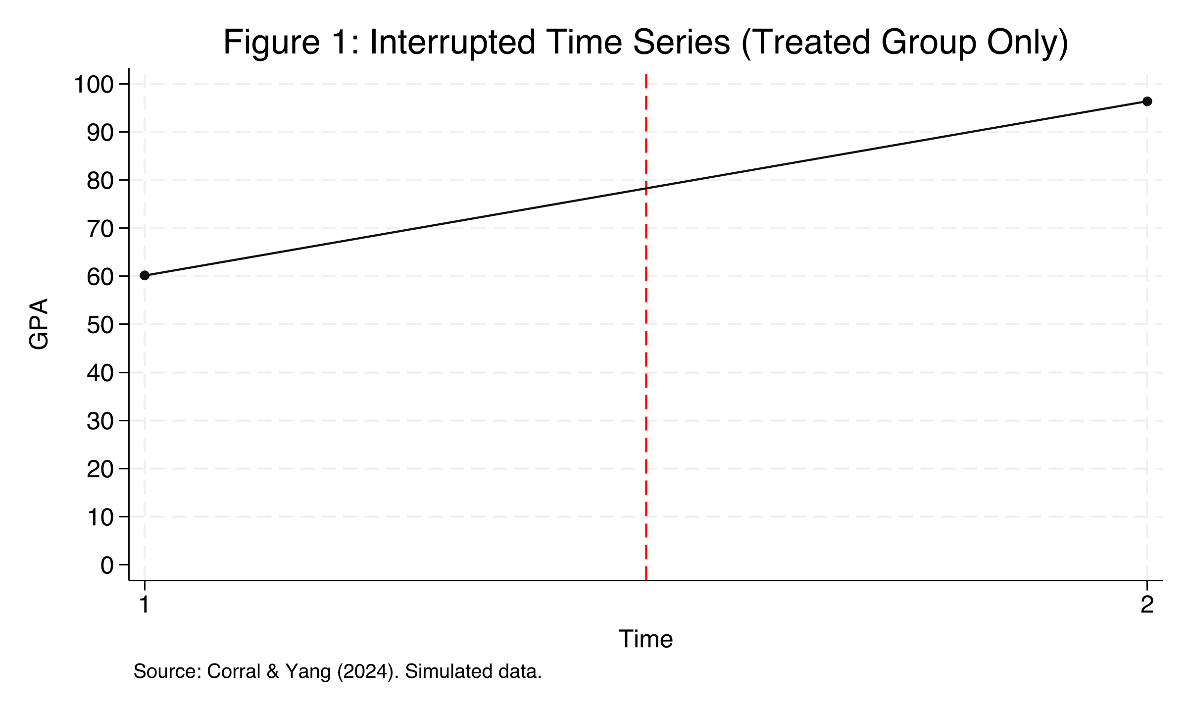
Look only at the treated schools and GPA jumps from 60 to 96. Spectacular. Or is something else rising too?

This is the central tension of policy evaluation without an RCT: a single-group before-after number conflates the program with everything else moving in time — maturation, grade inflation, district-wide reforms. The whole tutorial is about earning the right number out of this tempting wrong one.

The naive before-after answer is 36.20 — the credible answer is much smaller

Interrupted Time Series — treated schools only. GPA leaps across the red treatment line from ~60 to ~96.

Spoiler figure for Act I. Don’t reveal the DiD number yet — just plant that a single line, with no comparison group, cannot separate the program’s effect from the secular trend. We come back and net out that trend in Act II.

Where we’re going

• The naive ITS trap: before-after overstates the effect
• The 2×2 DiD design — a comparison group rebuilds the counterfactual
• Five equivalent Stata estimators land on one number
• The event study — testing parallel trends with pre-treatment leads

The Investigation

Act II

The lab: 35 schools, 2 periods, a clean simultaneous rollout

• Outcome — gpa, a school’s mean GPA on a 0–100 scale
• Treatment — 10 schools get tutoring; 25 are the comparison group
• Design — every treated school switches on at the same time (no staggering)

A strongly-balanced panel: 35 schools × 2 periods = 70 observations. The estimand is the ATT \(E[Y_i(1)-Y_i(0)\mid D_i=1]\) — the effect for the schools that actually got the program.

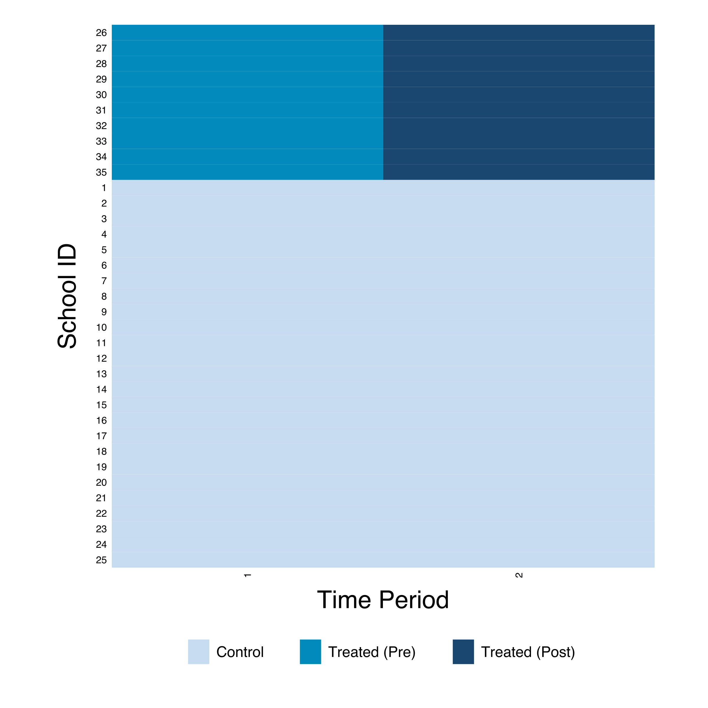
All 10 treated schools switch on together — the ideal 2×2 setup

Treatment-timing heatmap. Treated schools (IDs 26–35) flip pre → post simultaneously at time 2; the 25 comparison schools never switch.

panelview confirms there is no staggered adoption — the simplest, cleanest DiD case. This matters because staggered TWFE can produce biased estimates (Goodman-Bacon 2021); here that landmine is absent by construction, so the textbook 2×2 logic applies exactly.

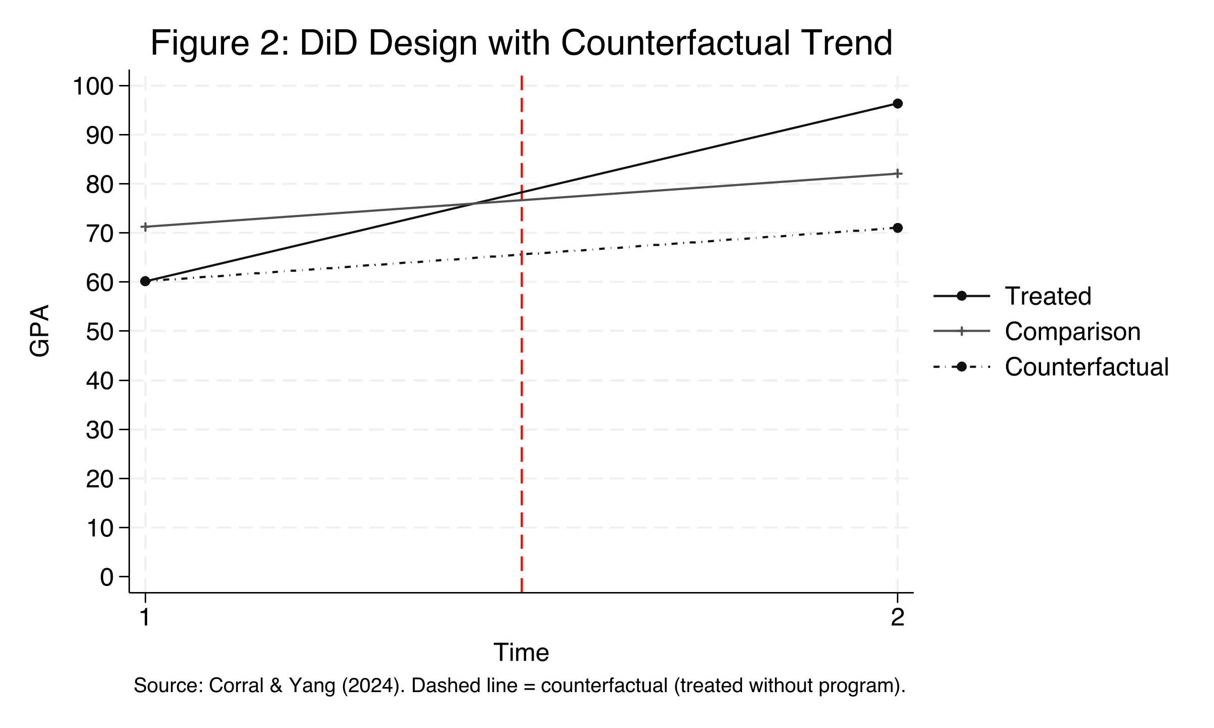
DiD rebuilds the counterfactual from the comparison group’s drift

The comparison group (rising gently) supplies the dashed counterfactual: where the treated would have ended up without the program.

Three lines: actual treated (60→96), comparison (71→82), and the counterfactual (60→71, dashed). The counterfactual is “treated pre-level + comparison’s pre-to-post change.” The vertical gap between the actual treated outcome and that dashed line is the DiD. This is the picture of the parallel-trends assumption.

Parallel trends: absent treatment, the two groups would have moved together

\[E[Y_{i,1}(0) - Y_{i,0}(0) \mid D=1] = E[Y_{i,1}(0) - Y_{i,0}(0) \mid D=0]\]

Different starting levels are fine. Different changes — divergent slopes — would break the design. This is the one assumption that does the causal work.

We can never observe the treated group’s untreated outcome in the post-period, so this is fundamentally untestable. What we CAN do is check pre-treatment trends — if the groups tracked each other before the program, the assumption is at least plausible. That check is the event study in Act III.

The double difference: subtract the comparison group’s trend from the treated group’s

\[DiD = \Big(\bar{Y}_{1}^{T} - \bar{Y}_{0}^{T}\Big) - \Big(\bar{Y}_{1}^{C} - \bar{Y}_{0}^{C}\Big)\]

Treated change \(36.20\) minus comparison change \(10.88\) = the program’s effect, with the common time trend removed.

Like two runners improving between races: if both were expected to improve from training, only the EXTRA improvement of the coached runner is the coaching effect. The comparison group’s 10.88 is the “training effect”; the remaining 25.32 is the “coaching effect” — the tutoring program.

The means table makes the subtraction explicit: 36.20 − 10.88 = 25.32

Group	Pre	Post	Change
Comparison (25 schools)	71.22	82.10	10.88
Treated (10 schools)	60.17	96.37	36.20
DiD estimate			25.32

Roughly one-third of the treated group’s raw gain (10.88 points) was natural drift, not the program.

Note the treated schools START lower (60.17 vs 71.22) — the program targeted schools with greater need. The pre-difference is −11.05; the post-difference is +14.27; the change in the gap, 25.32, is the ATT. This deficit-to-advantage reversal is the most compelling pattern in the data.

The formal diff command: ATT = 25.315, SE 0.627, p < 0.001

diff gpa, treated(treated) period(post)

Contrast	Estimate	SE	Sig.?
Before: Diff (T−C)	−11.049	0.443	yes
After: Diff (T−C)	14.266	0.443	yes
Diff-in-Diff	25.315	0.627	yes

The t-statistic is 40.40 — the effect is precisely estimated (R-squared 0.99, an artifact of simulated low-noise data). The reversal: treated schools were 11 points BELOW comparison before, and 14 points ABOVE after. Entirely attributable to the program under the DiD assumptions.

The same number as a regression: the interaction txp IS the DiD

\[Y_{it} = \alpha + \beta_1 \text{Treat}_i + \beta_2 \text{Post}_t + \beta_3 (\text{Treat}_i \times \text{Post}_t) + \varepsilon_{it}\]

reg gpa treated post txp, robust

\(\hat\beta_3 = 25.31\) (SE 0.61) — the DiD.

The rest is nuisance: constant 71.22 (comparison pre-mean), \(\hat\beta_1 = -11.05\) (baseline gap), \(\hat\beta_2 = 10.89\) (common trend).

Regression decomposes the DiD into building blocks and — crucially — lets you add controls, flexible standard errors, and extensions the manual subtraction cannot. The interaction coefficient is the entire causal payload; everything else is nuisance structure.

TWFE absorbs school and time effects; the interaction survives unchanged

\[Y_{it} = \beta_3 (\text{Treat}_i \times \text{Post}_t) + \gamma_i + \vartheta_t + \varepsilon_{it}\]

xtreg  gpa txp i.time, fe vce(cluster id)
reghdfe gpa txp, absorb(id time) cluster(id)

\(\gamma_i\) wipes out permanent school differences.

\(\vartheta_t\) wipes out common shocks. What remains: \(\hat\beta_3 = 25.31\).

Like a two-pass photo filter: the first pass removes school-specific stains (rich/poor, urban/rural), the second removes period-specific glare (a nationwide reform). reghdfe gives byte-identical results to xtreg but scales to large panels. Within R-squared 0.9946 — again, simulated-data clean.

Five estimators, one answer: 25.31–25.33 across the board

Method	Estimate	SE	Clustered?
diff (manual)	25.315	0.627	no
reg (interaction)	25.315	0.615	robust
didregress	25.315	0.834	yes
xtreg (TWFE)	25.315	0.585	yes
reghdfe (+ covariate)	25.328	0.605	yes

Adding the female-share control moves the estimate by ~0.01 points. The design — not the covariates — does the heavy lifting.

didregress (Stata 17+) labels its output ATET and auto-clusters at the school level, which is why its SE is the largest (0.834). The point estimate is rock-stable: in a well-designed DiD with proper fixed effects, covariates are cosmetic for identification. The differences are all in the standard errors, not the estimate.

The Resolution

Act III

The credible ATT is 25.32 GPA points — and the naive number overstated it by 43%

25.32

\(\hat\delta\), ATT (SE 0.627) · vs. naive ITS 36.20 — the 10.88-point gap was secular drift

This is the Act-I hook resolved. The naive 36.20 attributed all of the treated group’s gain to the program; DiD nets out the comparison group’s 10.88-point drift to recover 25.32. A policymaker using ITS alone would overstate the program’s effectiveness by 43%.

Do the leads look like zero? The event study tests parallel trends directly

\[Y_{it} = \alpha + \sum_{j=-m}^{q} \theta_j \cdot \text{treat}_{it}(t = k+j) + \gamma_i + \vartheta_t + \varepsilon_{it}\]

Replace the single interaction with one coefficient \(\theta_j\) per period relative to onset. Leads (\(j<0\)) test pre-trends; lags (\(j\geq 0\)) trace dynamics. The base period \(j=-1\) is omitted.

We switch to the expanded 8-period dataset (280 obs, treatment onset at period 5). The event study does double duty: pre-treatment leads near zero make parallel trends plausible, and post-treatment lags show whether the effect is immediate, ramps up, or fades.

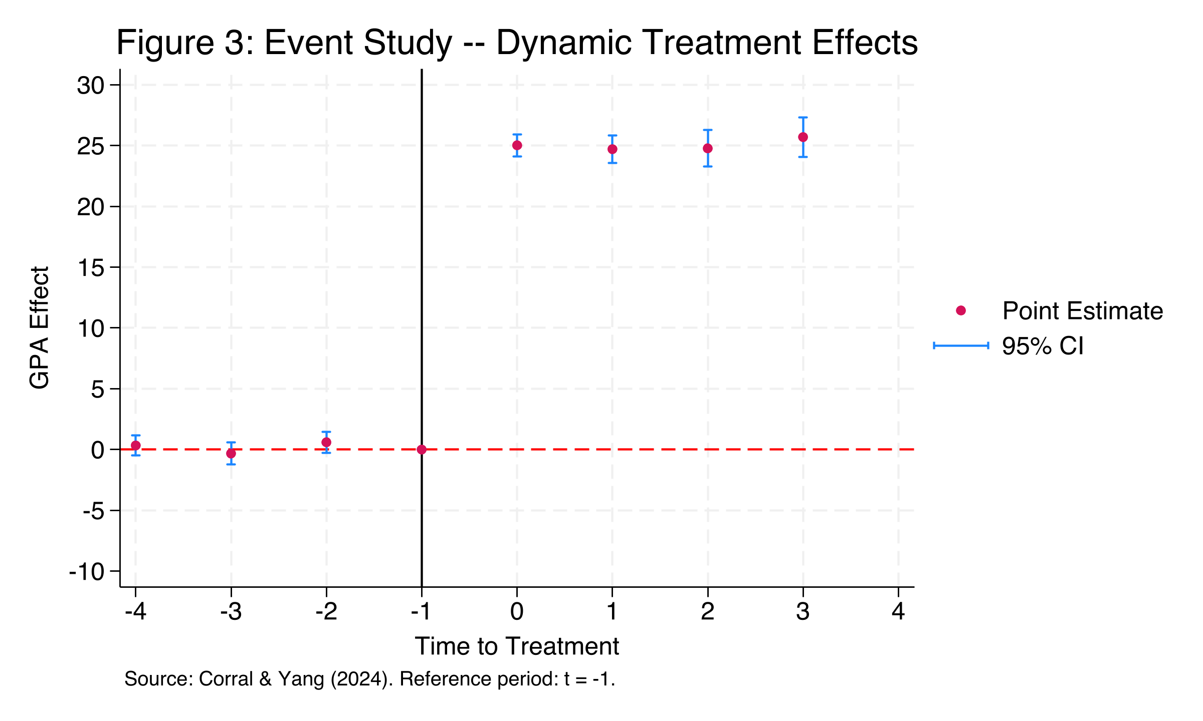
Flat pre-trends, then a sharp persistent jump — the identification check passes

Event study. Pre-treatment coefficients hug zero; at onset the effect leaps to ~25 and holds. Bands are 95% CIs.

The most informative figure in the analysis. The three visible leads are 0.34, −0.32, 0.59 — all insignificant (p = 0.40, 0.47, 0.17). That is the empirical signature of parallel pre-trends: treated and comparison schools moved together BEFORE the program. At onset the effect snaps to ~25 and stays there with tight CIs.

Leads near zero, lags near 25 — the table behind the picture

Period	Coefficient	SE	Sig.?
lead 4	0.342	0.401	no
lead 3	−0.322	0.441	no
lead 2	0.593	0.423	no
lag 0	25.028	0.445	yes
lag 1	24.705	0.559	yes
lag 2	24.768	0.739	yes
lag 3	25.701	0.797	yes

Lags span < 1 GPA point across four periods: no fade-out, no ramp-up — an immediate, sustained effect.

Pre-treatment leads range from −0.32 to 0.59, fluctuations well within sampling noise. Post-treatment lags range from 24.71 to 25.70 — remarkably flat. The program delivered its full benefit from period one and held it, consistent with a structural change in academic support rather than a temporary boost.

Does passing the pre-trends test make the result causal? Not by itself

Objection. Flat leads and five matching estimators still cannot prove the comparison group is a valid counterfactual.

Response. Correct. The ATT is identified only under parallel trends and SUTVA (no spillovers, consistent treatment). The event study is consistent with parallel trends — it never proves them. A failed pre-trend would refute the design; a passed one only fails to refute it.

Steelman, don’t strawman. Falsely-reassuring perfect pre-trends here are a feature of simulated data; real applications are noisier. And the data are pedagogical — a 25-point gain on a 100-point scale is far larger than real after-school programs (typically 0.1–0.3 SD). For staggered rollouts, prefer Callaway–Sant’Anna or Sun–Abraham over plain TWFE.

Let the comparison group, not the calendar, tell you what the program did.

The single takeaway. A credible comparison group plus a parallel-trends check is what separates a believable 25.32 from a misleading 36.20. The design does the causal work; the five estimators and the covariate are just confirmation.