Do Institutions Cause Prosperity?

An instrumental-variables tutorial in Stata — replicating Acemoglu, Johnson & Robinson (2001)

0.9442SLS effect of institutions

+81%larger than OLS (0.522)

16.32first-stage F · 64 ex-colonies

Carlos Mendez

Nagoya University (GSID)

June 11, 2026

The Tension

Act I

Richer countries have better institutions — but which way does the arrow point?

Stronger property-rights institutions track vastly higher income across countries. The slope is real and huge.

But correlation is not causation. Maybe rich countries simply afford better courts. Maybe geography or culture drives both. Which way does the arrow point?

This is the central problem of development economics. The cross-country plot of institutions vs income has a clean positive slope, but three threats contaminate it: reverse causality (rich countries can afford institutions), omitted variables (geography, culture, human capital), and measurement error in the institutional index. None of these can be settled by staring at the scatter harder.

A deadly natural experiment: where Europeans died, extractive institutions followed

Acemoglu, Johnson & Robinson (2001) use European settler mortality during colonization as an instrument for modern institutions.

Tropical, disease-ridden colonies → Europeans died → extractive rule. Temperate, survivable colonies → Europeans settled → property-rights institutions.

The AJR argument: settler mortality circa 1500–1900 was driven by malaria and yellow fever, not by 1995 income. Places where Europeans died en masse became extractive colonies designed to ship resources home; places where they survived got European-style institutions. That historical accident is the source of exogenous variation in institutions we can exploit.

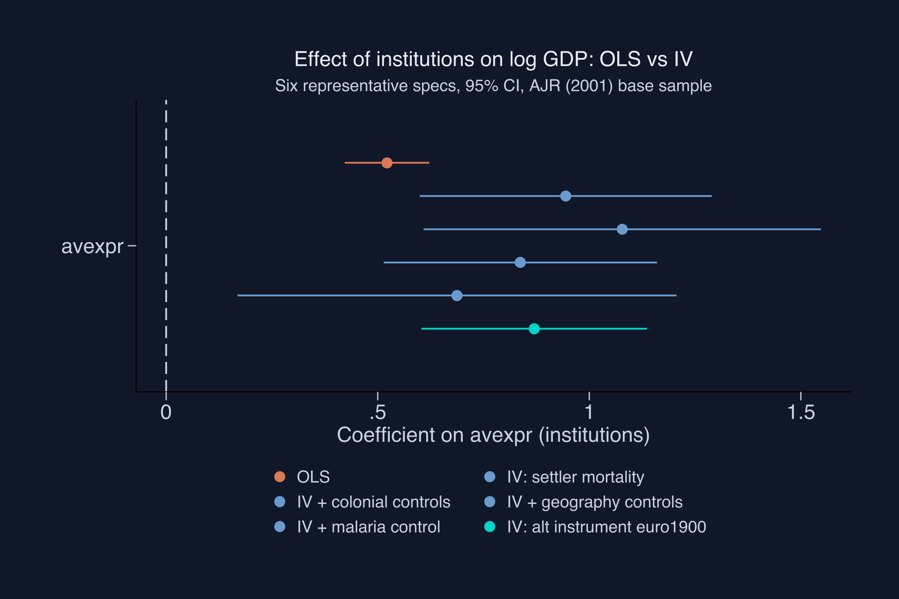
Five estimates, one dataset: OLS says 0.52, IV says 0.94

Coefficient on institutions across six specs — OLS (orange), four IV variants with settler mortality (steel), IV with an alternative instrument (teal). 95% CIs.

Spoiler figure — we earn each estimate in Act II. Don’t explain every bar yet. Just plant the headline: the naive OLS slope (orange) sits at 0.52 with a tight CI, while every IV variant (steel/teal) lives in the 0.7–1.0 band. The gap between orange and blue is the whole story.

Where we’re going

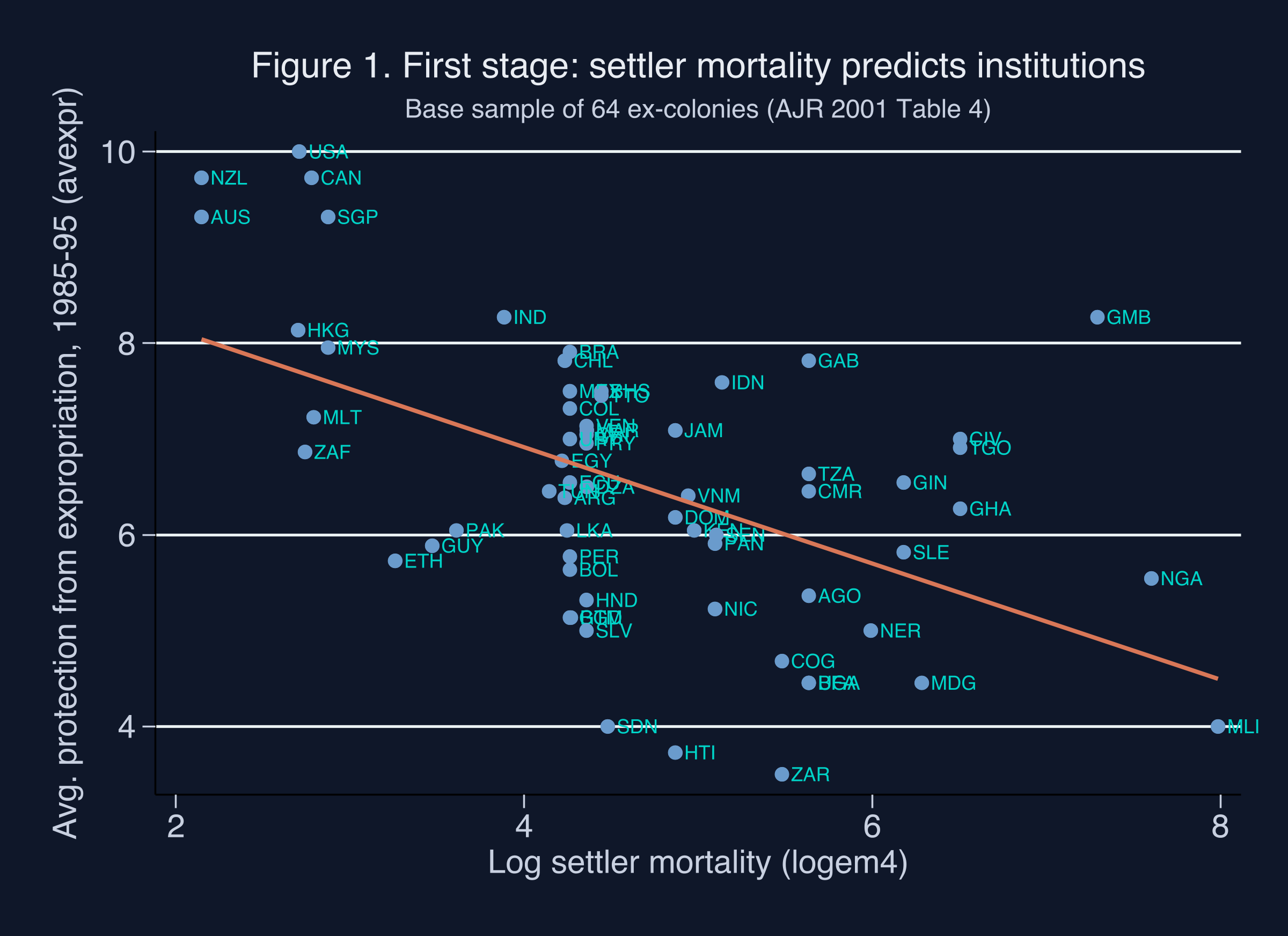
• The instrument: settler mortality across 64 ex-colonies
• The three conditions an instrument must satisfy
• 2SLS = reduced form ÷ first stage
• The headline: institutions raise GDP by 0.944 (a LATE)
• Five families of robustness — and the one honest doubt

The Investigation

Act II

A regressor correlated with the error term makes OLS lie

\[Y_i = \alpha + \beta X_i + U_i, \quad \text{with} \;\; \mathrm{Cov}(X_i, U_i) \neq 0\]

\(Y\) is log GDP, \(X\) is institutional quality, \(U\) collects every unobserved driver of income. The non-zero covariance is exactly what biases OLS.

This is endogeneity in one line. Institutions are endogenous because they are jointly determined with GDP, share confounders with GDP (geography, culture, human capital), and are measured with noise. OLS of Y on X does not recover beta even in infinite samples. The Durbin-Wu-Hausman test later confirms the endogeneity is real, not just assumed.

An instrument must clear three bars: relevance, exclusion, exogeneity

• Relevance — \(Z\) moves \(X\). Testable (first-stage F).
• Exclusion — \(Z\) affects \(Y\) only through \(X\). Untestable.
• Exogeneity — \(Z\) is uncorrelated with \(U\). Untestable.

Settler mortality must shift institutions (we can check) and reach 1995 GDP only through them (we must assume).

Relevance is the one condition data can verify — the first-stage F-statistic. Exclusion and exogeneity are the heart of every IV paper and are assumptions, not findings. AJR’s substantive claim is that 1700-era mortality cannot touch 1995 income except by shaping the institutions countries inherited. Overidentification (Hansen J) can partially probe this, but never prove it.

2SLS sieves out the contaminated variation, then runs OLS on what passes

\[\hat\beta_{2SLS} = \frac{\widehat{\mathrm{Cov}}(Y, Z)}{\widehat{\mathrm{Cov}}(X, Z)} = \frac{\hat\beta_{RF}}{\hat\beta_{FS}}\]

Stage 1 regresses \(X\) on \(Z\); stage 2 regresses \(Y\) on the predicted \(\hat X\). With one instrument, the IV estimate is just reduced form \(\div\) first stage.

The sieve analogy: stage 1 catches the dirt (the confounded part of institutions), and only the clean signal — the part of X predicted by the instrument — passes through to stage 2. ivreg2 does both stages internally and reports correct second-stage standard errors. Crucially the ratio identity below makes IV concrete: it is one division.

OLS first: with zero controls, institutions “explain” a 0.522 slope

Sample	\(\hat\beta\) (avexpr)	SE	Sig. 1%?
Full (N=111)	0.532	0.029	yes
Base (N=64)	0.522	0.050	yes
+ continents	0.390	0.051	yes

This is the number the IV will stress-test — not one it generates.

The naive OLS slope is remarkably stable: 0.53 full sample, 0.52 base sample, falling only to 0.39 with continent dummies. A one-point rise in expropriation protection (0–10 scale) is associated with a 39–53% income gain. But three biases lurk: reverse causality and omitted variables push it up, measurement error pulls it down. We need IV to decompose 0.522 into bias plus true effect.

First stage: deadlier colonies inherited weaker institutions (slope −0.607)

Modern expropriation protection vs log settler mortality, 64 ex-colonies. Slope \(= -0.607\), \(F = 16.32\), \(R^2 = 0.27\).

Relevance, visualized. Australia, New Zealand, the USA — the lowest-mortality colonies — sit at avexpr ≈ 9–10. Sierra Leone, Niger, Mali — among the deadliest — sit near 3.5–5. A one-log-point rise in mortality lowers institutions by 0.607 (t = 4.04). The fit captures 27% of institutional variation. This is the empirical engine of the whole IV.

Is the instrument strong enough? F = 16.32 — passing, but barely

Diagnostic	Value	Threshold
Kleibergen-Paap rk Wald F	16.32	10 (rule of thumb)
Stock-Yogo 10% max IV size	—	16.38 (iid)
Anderson-Rubin Wald (robust)	61.66	\(p < 0.0001\)

Borderline on the conventional threshold; the weak-IV-robust AR test reassures.

Honest disclosure: 16.32 vs the Stock-Yogo iid threshold of 16.38 is essentially a wash. It clears the Staiger-Stock F > 10 rule of thumb but sits right at the more refined bar. Under robust SEs the right benchmark is the Olea-Pflueger effective F (weakivtest). The Anderson-Rubin Wald test (F = 61.66) is weak-IV-robust and confirms significance even if you distrust conventional 2SLS asymptotics on a borderline F.

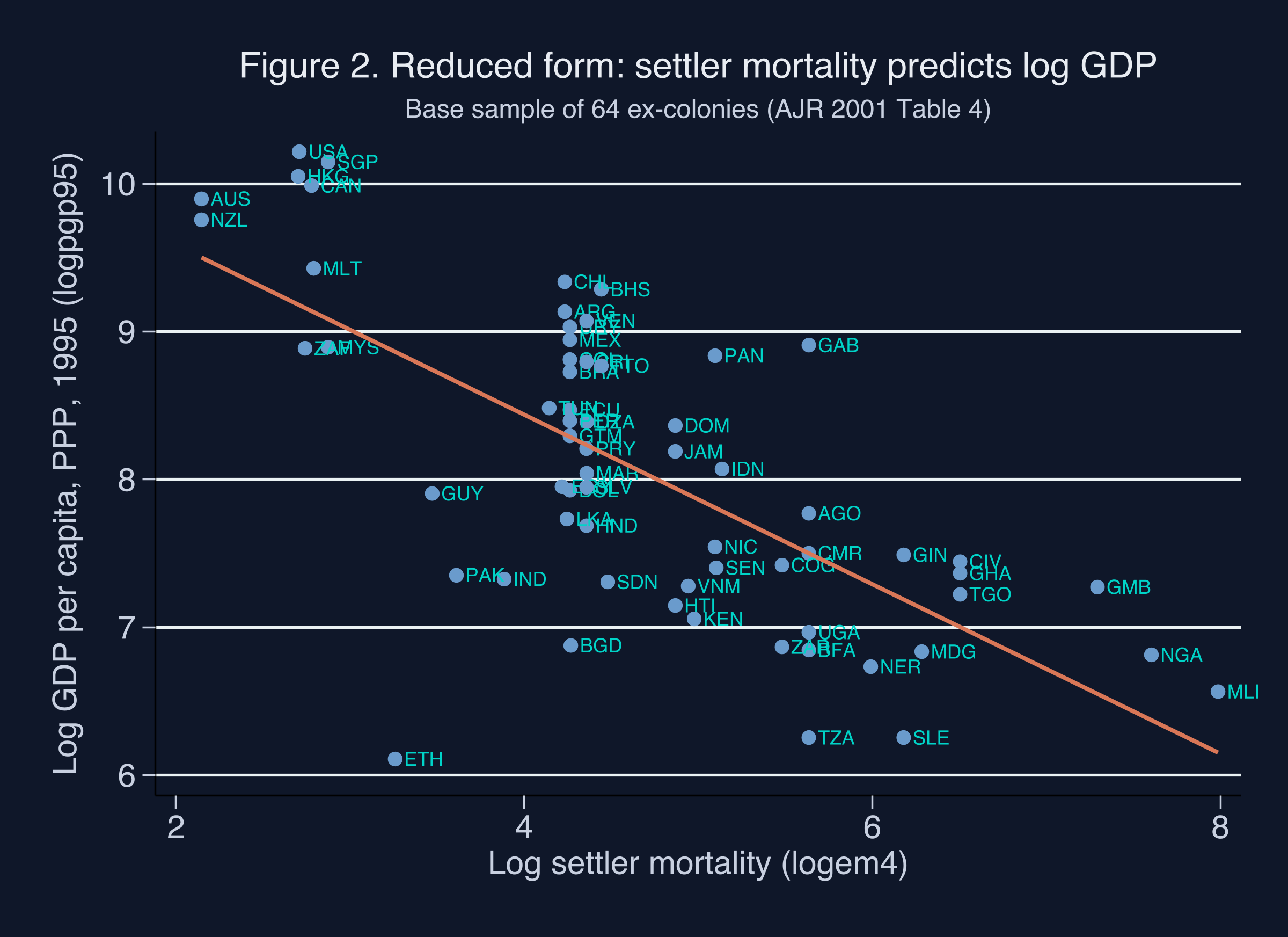
Reduced form: the instrument’s total reach on income is steep

Log GDP per capita (1995, PPP) vs log settler mortality, 64 ex-colonies. Slope \(\approx -0.573\).

The reduced form regresses the outcome directly on the instrument, skipping institutions. Across the 5.8-log-point span of mortality the fitted line predicts a GDP gap of about 3.4 log points — the highest-mortality colonies roughly 30x poorer than the lowest. This is the total effect of Z on Y. The IV decomposes it: divide this −0.573 by the first-stage −0.607 and you get 0.944.

Six lines of Stata estimate the whole IV

use "maketable4.dta", clear
keep if baseco==1
ivreg2 logpgp95 (avexpr = logem4), ///
    robust first endog(avexpr)

(avexpr = logem4) declares the endogenous regressor and its instrument; endog() runs the Durbin-Wu-Hausman test.

ivreg2 is the IV workhorse from SSC. The parenthetical syntax (endogenous = instrument) is the whole IV declaration. first prints the first-stage F; endog(avexpr) triggers the Durbin-Wu-Hausman endogeneity test. robust gives heteroskedasticity-consistent SEs throughout. The full do-file runs all of Tables 1–8; these are the load-bearing lines.

The Resolution

Act III

Instruments raise the institutional effect to 0.944

0.944

2SLS coefficient on institutions (robust SE 0.176) · 81% larger than OLS · \(z = 5.36\)

The headline. 2SLS = 0.944, robust SE 0.176, 95% CI [0.60, 1.29], significant at 1%. It is 81% larger than the OLS 0.522. The reduced-form ÷ first-stage identity (−0.573 / −0.607) reproduces it exactly. In domain terms, lifting Nigeria’s institutions to Chile’s level would raise its log GDP by ≈ 2.15 points — an 8.5-fold income increase. Enormous, and a LATE.

The IV > OLS gap reveals measurement error, not reverse causality

Estimator	\(\hat\beta\)	SE	vs OLS
OLS	0.522	0.050	—
2SLS	0.944	0.176	+81%

Durbin-Wu-Hausman \(\chi^2 = 9.09\) (\(p = 0.003\)) rejects OLS consistency.

Three biases pull in opposite directions: reverse causality and omitted variables push OLS up, classical measurement error pulls it down. IV being LARGER than OLS implies the downward (attenuation) bias dominates — the institutional index is a noisy proxy for the true property-rights regime, and de-noising it via IV reveals a steeper causal slope. The endogeneity test confirms the gap is statistical, not noise: OLS is genuinely biased here.

The effect survives 27 control sets — institutions in the 0.7–1.0 band

• Colonial / legal / religion (Tab 5): 0.92–1.34
• Geography / climate (Tab 6): 0.71–1.36
• Health channels (Tab 7): 0.55–0.69 — the only dip toward OLS

No control set drives the coefficient to zero or flips its sign.

Across 27 specifications the institutional coefficient stays in the 0.55–1.36 range with the 0.944 baseline near the middle. British/French dummies, legal origin, religion shares, temperature, humidity, minerals, landlock, ethnolinguistic fractionalization — none kill it. The health-channel specs (malaria, life expectancy, infant mortality) are the only place it approaches OLS, and there the first-stage F collapses below 5, so read those CIs not point estimates.

The strongest objection — and the honest answer

Objection. Maybe settler mortality still depresses 1995 income directly — through malaria and disease — violating the exclusion restriction.

Response. Add health controls and the effect dips to 0.55–0.69. But there the first-stage F falls to 1.2–4.9 (weak IV), and Hansen J fails to reject (\(p = 0.46\)–\(0.76\)). The doubt is real; it is the place to keep an open mind.

Steelman, don’t strawman. Health is the tightest threat to exclusion. AJR’s reading: modern health is a “bad control” — itself an outcome of institutions, so adjusting for it shrinks the coefficient artifactually. A critic’s reading: disease is a genuine direct channel. The data cannot adjudicate. Add Albouy (2012): ~36% of mortality observations are imputed or shared, so Hansen J non-rejection has low power against shared imputation noise. Honesty over comfort.

What 0.944 is — and is not: it is a LATE, not an ATE

What it IS

• effect for compliers
• countries whose institutions would shift with mortality history
• a real effect on real countries

What it is NOT

• a population ATE
• a claim about every country
• proof — exclusion stays an assumption

Under heterogeneous effects (Imbens-Angrist 1994), 2SLS identifies the Local Average Treatment Effect — the effect on compliers, the subpopulation whose institutional quality would have changed had their settler-mortality history been different. It is silent on never-colonized states or established democracies far from the colonization margin. LATE = ATE only under constant effects. And the exclusion restriction remains untestable in principle.

Institutions are roughly twice as valuable as naive regressions suggest

If the causal effect is 0.944, not 0.522, then institutional reform is about twice as powerful a lever as OLS implies.

Naive policy advice built on OLS slopes systematically understates the returns to building courts, regulators, and parliaments.

The practical payoff. Measurement error means OLS understates the returns to institutions by ~80%. For policymakers, reforms that look merely correlated with growth in OLS samples may be substantially more powerful causal levers. The academic caveats (LATE, exclusion, Albouy) sharpen the claim without overturning it: the direction and rough magnitude are robust.

Let the historical accident, not the naive regression, reveal the causal slope.

The single takeaway. A 1700-era natural experiment in settler mortality, used as an instrument, lifts the estimated effect of institutions on prosperity from 0.522 to 0.944 — and that gap is the measurement error OLS could never see. IV recovers a LATE under an untestable exclusion restriction, but the lesson is durable: when X is endogenous, find the exogenous nudge and let it do the identifying.