IV Estimation with Panel Data: Economic Shocks and Civil Conflict
Abstract
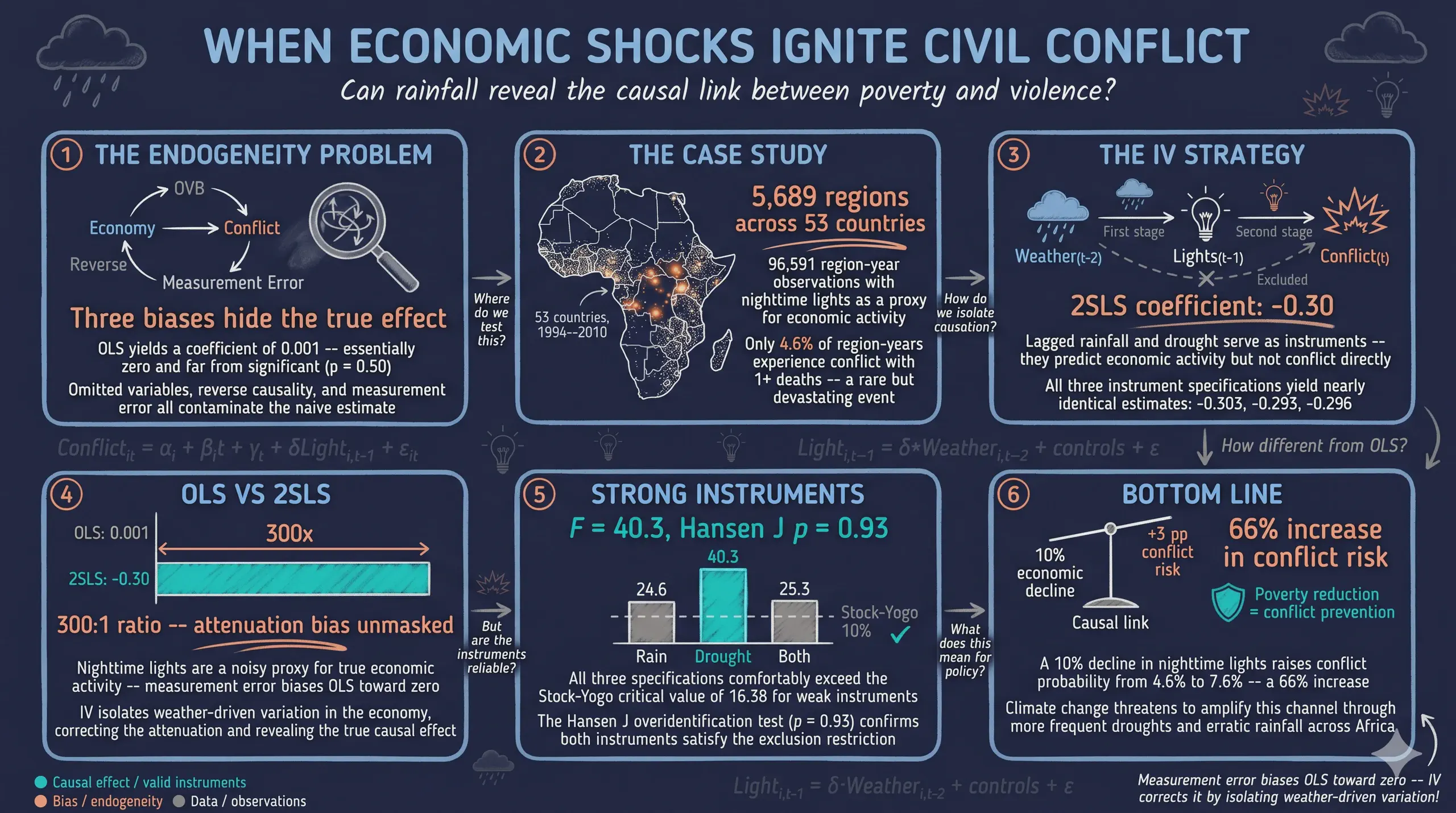
The correlation between economic deprivation and civil conflict is well documented, but correlation is not causation: omitted confounders, reverse causality, and measurement error in proxies for local income all threaten any naive regression of conflict on economic activity. This tutorial sets out to estimate the causal effect of economic shocks on civil conflict by replicating and extending Hodler and Raschky (2014), who took the rainfall-as-instrument strategy of Miguel, Satyanath, and Sergenti (2004) to the subnational level. The data comprise 96,591 region-year observations from 5,689 administrative regions across 53 African countries over 1994–2010, where conflict is measured as a binary outcome (1+ or 25+ deaths), nighttime light intensity proxies economic activity, and lagged rainfall and the Palmer Drought Severity Index serve as instruments. Using Stata’s xtreg and xtivreg2, the analysis runs fixed-effects OLS, reduced-form, and 2SLS/IV estimation with region-specific trends, year effects, and clustered standard errors. OLS returns a near-zero coefficient of 0.001 (p = 0.50), whereas 2SLS yields −0.296 (SE 0.076, p < 0.01) using both instruments, a roughly 300-fold gap consistent with attenuation bias. A 10% decline in economic activity raises the probability of conflict by about 3 percentage points—a 66% increase over the 4.6% baseline—with strong first-stage F-statistics (24.62–40.33, above the Stock-Yogo threshold of 16.38) and a Hansen J p-value of 0.932 confirming instrument strength and validity. The results imply that poverty reduction is conflict prevention, underscoring the security implications of climate-driven economic shocks.
1. Overview
Does poverty cause violence? This is one of the most important questions in development economics — and one of the hardest to answer. The correlation between economic deprivation and civil conflict is well documented, but correlation is not causation. Poor regions may experience more conflict for reasons unrelated to their poverty, or conflict itself may destroy economic activity, creating reverse causality.
In a landmark contribution, Miguel, Satyanath, and Sergenti (2004) proposed a clever solution: use rainfall as an instrument for economic shocks. The logic is simple — rain affects agricultural output, agricultural output affects incomes, and incomes affect the incentives for violence. But rain itself is plausibly random, meaning it can isolate the causal direction from economics to conflict.
This tutorial replicates and extends the analysis of Hodler and Raschky (2014), who took this approach to the subnational level. Instead of comparing countries, they compared 5,689 administrative regions across 53 African countries, using nighttime light intensity as a proxy for economic activity and lagged rainfall and drought as instrumental variables. Their finding: negative economic shocks significantly increase the probability of civil conflict.
We will walk through the complete IV estimation workflow in Stata — from descriptive statistics, through reduced-form and OLS estimates, to 2SLS/IV estimation with first-stage diagnostics. Along the way, we will learn why OLS produces biased estimates, how instruments fix this, and what diagnostic tests to check.
Learning objectives
- Understand the endogeneity problem in studying economic shocks and conflict
- Implement fixed-effects panel regression with
xtregin Stata - Estimate 2SLS/IV models using
xtivreg2with panel data - Interpret first-stage F-statistics and the Stock-Yogo weak instrument test
- Evaluate instrument validity using the Hansen J overidentification test
- Compare OLS and 2SLS estimates and explain the attenuation bias from measurement error
- Visualize first-stage relationships with binned scatter plots
Key concepts at a glance
The post leans on a small vocabulary repeatedly. The rest of the tutorial assumes you can move between these terms quickly. Each concept below has three parts. The definition is always visible. The example and analogy sit behind clickable cards: open them when you need them, leave them collapsed for a quick scan. If a later section mentions “exclusion restriction” or “Stock-Yogo” and the term feels slippery, this is the section to re-read.
1. Endogeneity. A regressor is endogenous if it correlates with the error term. The OLS slope is then a contaminated mix of the causal effect and the bias from omitted confounders, simultaneity, or measurement error. Endogeneity is the headline reason simple regressions can mislead.
Example
In this post llnlight01 (lagged nighttime light intensity, the proxy for local economic activity) is endogenous in the conflict regression. Conflict suppresses light AND light measures activity that conflict reflects — reverse causality plus measurement error. OLS returns 0.001 (p = 0.50). The IV estimate flips sign and grows.
Analogy
A contaminated thermometer. The thermometer has two sources of contamination: it is held by the patient (reverse causality) and it is corroded (measurement error). Reading off the temperature gives nonsense.
2. Instrumental variable $Z$. An external variable that drives variation in the endogenous regressor without belonging in the outcome equation. Two requirements: $Z$ must predict the regressor (relevance) and $Z$ must affect $Y$ only through the regressor (exclusion).
Example
This post uses two instruments for llnlight01: lagged log rainfall (l2lnrain01) and lagged Palmer Drought Severity Index (l2meanpdsi). Weather is plausibly exogenous to current conflict, but it shifts agricultural output and hence economic activity (light).
Analogy
A clean thermometer that the contamination cannot reach. The instrument lives outside the contaminated system. Its readings on the regressor are clean. We use them to back out the temperature.
3. Relevance and the first stage. The first stage is the regression of the endogenous regressor on the instruments and controls. Relevance is the requirement that the instruments significantly predict the regressor in the first stage. The first-stage F-statistic measures instrument strength.
Example
First-stage F is 24.62 with rainfall alone, 40.33 with drought alone, and high in the joint specification. Both single-instrument F-stats clear the conventional weak-instrument threshold of 10 by a wide margin.
Analogy
The clean thermometer has to be sensitive enough. A thermometer that barely moves is useless. The first-stage F is the calibration test: does the clean thermometer respond strongly to the underlying signal?
4. Exclusion restriction. The assumption that the instrument $Z$ affects the outcome $Y$ only through the endogenous regressor. No direct effect of $Z$ on $Y$. The exclusion restriction is the most contested part of any IV design — it is fundamentally untestable when there is exactly one instrument.
Example
For rainfall to be a valid instrument, lagged rainfall must affect conflict only through its effect on local economic activity. Direct effects (e.g. rain washing out a battlefield) would violate exclusion. The post discusses why African settings make this assumption defensible.
Analogy
The clean thermometer is not also being heated by something else. If a hidden flame is warming the thermometer directly, its reading no longer maps cleanly to the patient’s temperature. Exclusion is “no other heat source on the instrument.”
5. Stock-Yogo weak-IV test. A formal test for weak instruments. The test compares the first-stage F-statistic against a critical value chosen to bound the bias of 2SLS at, e.g., 10% of OLS bias. With one endogenous regressor and one instrument, the rule-of-thumb critical value is 16.38 for the 10% maximal IV size criterion.
Example
The post compares F = 24.62 (rainfall) and F = 40.33 (drought) against the Stock-Yogo critical value of 16.38. Both clear the bar comfortably. The instruments are not weak.
Analogy
How sensitive does the thermometer have to be before its reading is trustworthy? Stock-Yogo gives the answer in numbers. Below the threshold, even a “significant” first stage produces unreliable IV estimates.
6. 2SLS — Two-Stage Least Squares. The standard IV estimator. Stage 1: regress the endogenous variable on instruments and controls; obtain fitted values. Stage 2: regress the outcome on the fitted endogenous variable and controls. The second-stage slope is the IV estimate of the causal effect.
Example
All four IV columns in this post use 2SLS via Stata’s xtivreg2. The headline 2SLS estimate using both instruments is -0.296 (SE 0.076, p < 0.01). A one-unit increase in log nighttime light intensity reduces the conflict probability by ~0.30 percentage points.
Analogy
Take two readings and combine. Stage 1 calibrates the clean thermometer to the contaminated one. Stage 2 reads off the patient’s temperature using the calibrated mapping. Two careful steps replace one careless one.
7. Hansen J overidentification test. A joint test of instrument validity when there are more instruments than endogenous regressors. The J-statistic checks whether the multiple instruments give consistent answers; failing the test signals at least one instrument is invalid (likely violating exclusion).
Example
With two instruments (rainfall, drought) and one endogenous regressor (llnlight01), the system is overidentified by one degree. The Hansen J p-value is 0.932 — far from rejection. The two instruments tell the same story. Joint validity is plausible.
Analogy
Compare two clean thermometers. If both report the same temperature, you trust the reading more. If they disagree wildly, at least one is broken — but you don’t know which. The Hansen test is “do the clean thermometers agree?”
8. Attenuation bias. Classical measurement error in a regressor produces downward bias toward zero in OLS. The slope is shrunk by the noise-to-signal ratio. IV with a clean instrument removes the bias and typically returns a larger estimate (in absolute value).
Example
OLS on this dataset returns 0.001 (essentially zero). 2SLS returns -0.296 to -0.303 — two orders of magnitude larger and with the opposite sign. The OLS estimate was a small, contaminated reading; the IV estimates are the clean signal.
Analogy
The contaminated thermometer reads 37.0°C when the patient is at 38.5°C. The contamination shrinks the deviation toward the average. IV cleans the contamination and reveals the larger underlying difference.
2. The endogeneity problem
Why can’t we simply regress conflict on economic activity? The diagram below illustrates the three threats to identification.
graph TD
    ECON["<b>Economic Activity</b><br/>(Nighttime lights)"]
    CONF["<b>Civil Conflict</b>"]
    U["<b>Unobservables</b><br/>(Institutions, geography,<br/>ethnic fractionalization)"]
    ME["<b>Measurement Error</b><br/>(Lights ≠ true GDP)"]
    REV["<b>Reverse Causality</b><br/>(Conflict destroys<br/>infrastructure)"]

    ECON -->|"Causal effect?"| CONF
    U -->|"Omitted variable bias"| ECON
    U -->|"Omitted variable bias"| CONF
    CONF -->|"Reverse causality"| ECON
    ME -->|"Attenuation bias"| ECON

    style ECON fill:#6a9bcc,stroke:#141413,color:#fff
    style CONF fill:#d97757,stroke:#141413,color:#fff
    style U fill:#141413,stroke:#d97757,color:#fff
    style ME fill:#141413,stroke:#6a9bcc,color:#fff
    style REV fill:#141413,stroke:#00d4c8,color:#fff
Three problems arise when estimating the causal effect of economic shocks on conflict with OLS:
- Omitted variable bias — Unobserved factors like institutional quality, ethnic diversity, or geography may simultaneously affect both economic activity and conflict.
- Reverse causality — Conflict destroys infrastructure and economic activity, making it hard to know which direction the causal arrow runs.
- Measurement error — Nighttime light intensity is a proxy for true economic activity. Classical measurement error in the explanatory variable biases the OLS coefficient toward zero (attenuation bias).
The instrumental variables strategy addresses all three problems simultaneously. We need instruments that (a) predict economic activity (relevance) but (b) affect conflict only through their effect on economic activity (exclusion restriction).
3. The IV strategy
Hodler and Raschky (2014) use lagged rainfall and lagged drought intensity as instruments for nighttime light intensity. The identification relies on a simple lag structure:
graph LR
    W["<b>Weather(t-2)</b><br/>Rain / Drought"]
    L["<b>Light(t-1)</b><br/>Economic activity"]
    C["<b>Conflict(t)</b>"]

    W -->|"First stage"| L
    L -->|"Second stage"| C
    W -.->|"Excluded"| C

    style W fill:#6a9bcc,stroke:#141413,color:#fff
    style L fill:#d97757,stroke:#141413,color:#fff
    style C fill:#00d4c8,stroke:#141413,color:#141413
Weather in year $t-2$ affects economic activity in year $t-1$ (the first stage), and economic activity in year $t-1$ affects conflict in year $t$ (the second stage). The exclusion restriction requires that weather in $t-2$ has no direct effect on conflict in $t$ other than through economic activity — a plausible assumption given the two-year lag.
The structural model (second stage) is:
$$ Conflict_{it} = \alpha_i + \beta_i t + \gamma_t + \delta \cdot Light_{i,t-1} + \epsilon_{it} $$
where $\alpha_i$ are region fixed effects, $\beta_i t$ are region-specific time trends, and $\gamma_t$ are year fixed effects. The parameter of interest is $\delta$ — the causal effect of economic activity on conflict probability.
The first stage is:
$$ Light_{i,t-1} = \widetilde{\alpha}_i + \widetilde{\beta}_i t + \widetilde{\gamma}_t + \widetilde{\delta} \cdot Weather_{i,t-2} + \widetilde{\epsilon}_{it} $$
where $Weather_{i,t-2}$ can be rainfall, drought (Palmer Drought Severity Index), or both.
Estimand: The parameter $\delta$ is the Local Average Treatment Effect (LATE) — the causal effect of economic shocks on conflict for regions whose economic activity is affected by weather variation. This is the population of “compliers” in the IV framework.
4. Data loading and exploration
The dataset contains 96,591 region-year observations from 5,689 subnational administrative regions across 53 African countries, with yearly data from 1994 to 2010.
use "reference/EL_regional_conflict_replication.dta", clear
tsset objectid year
describe
Contains data from reference/EL_regional_conflict_replication.dta
 Observations:        96,591
    Variables:            14

Variable      Storage   Display    Value
    name         type    format    label      Variable label
-------------------------------------------------------------------------------
objectid        long    %12.0g                Value
year            float   %9.0g
countrycode     str3    %9s                   ISO
countryname     str32   %32s                  NAME_0
ucdp_death_du~y float   %9.0g                 Conflict (>1 deaths)
ucdp_25death_~y float   %9.0g                 Conflict (>25 deaths)
llnlight01      float   %9.0g                 Ln Lights(t-1)
l2lnrain01      float   %9.0g                 Ln Rain(t-2)
l2meanpdsi      float   %9.0g                 (Non) Drought(t-2)
ucdp_death_du~t float   %9.0g                 Conflict (>1 deaths)
ucdp_25death_~t float   %9.0g                 Conflict (>25 deaths)
llnlight01_dt   float   %9.0g                 Ln Lights(t-1)
l2lnrain01_dt   float   %9.0g                 Ln Rain(t-2)
l2meanpdsi_dt   float   %9.0g                 (Non) Drought(t-2)
The dataset includes both raw variables and pre-detrended versions (the *_dt suffix). The detrended variables are residuals from region-specific linear time trends — equivalent to including region-specific trends in the regression. We use the detrended variables throughout, following the original paper.
Variables
| Variable | Description | Type |
|---|---|---|
objectid | Region identifier | Panel ID |
year | Year (1994–2010) | Time variable |
ucdp_death_dummy | Conflict with 1+ deaths in region-year | Binary (outcome 1) |
ucdp_25death_dummy | Conflict with 25+ deaths in region-year | Binary (outcome 2) |
llnlight01 | Log nighttime light intensity (t-1) | Continuous (endogenous) |
l2lnrain01 | Log rainfall (t-2) | Continuous (instrument 1) |
l2meanpdsi | Palmer Drought Severity Index (t-2) | Continuous (instrument 2) |
5. Descriptive statistics
Let us examine the key variables to understand the data before estimation.
summarize ucdp_death_dummy ucdp_25death_dummy llnlight01 l2lnrain01 l2meanpdsi
    Variable |        Obs        Mean    Std. dev.       Min        Max
-------------+---------------------------------------------------------
ucdp_death~y |     96,591    .0455425    .2084919          0          1
ucdp_25dea~y |     96,591    .0144527    .1193481          0          1
  llnlight01 |     96,591   -1.611658    2.619427   -4.60517   4.143293
  l2lnrain01 |     96,591      3.8302    1.477743   -4.60517   6.093216
  l2meanpdsi |     96,591   -1.215386    2.033711   -12.1292    12.6313
Conflict is a rare event: only 4.6% of region-year observations experience at least one conflict-related death, and only 1.4% experience 25 or more deaths. The nighttime light variable (logged, lagged one year) averages -1.61, reflecting the low light intensity in most African regions — many areas are effectively dark. The mean PDSI of -1.22 indicates that the average region leans slightly toward dry conditions.
The panel decomposition reveals how much variation is between regions versus within regions over time.
xtsum ucdp_death_dummy ucdp_25death_dummy llnlight01 l2lnrain01 l2meanpdsi
Variable         |      Mean   Std. dev.       Min        Max |    Observations
-----------------+--------------------------------------------+----------------
ucdp_d~y overall |  .0455425   .2084919          0          1 |     N =   96591
         between |             .1176404          0          1 |     n =    5689
         within  |             .1721562  -.8956339    .986719 | T-bar = 16.9786

llnli~01 overall | -1.611658   2.619427   -4.60517   4.143293 |     N =   96591
         between |             2.568635   -4.60517   4.140281 |     n =    5689
         within  |             .5277626  -7.699739   2.693339 | T-bar = 16.9786

l2lnr~01 overall |    3.8302   1.477743   -4.60517   6.093216 |     N =   96591
         between |             1.493749   -4.60517   5.514849 |     n =    5689
         within  |             .1993702  -2.741027   5.494656 | T-bar = 16.9786
The decomposition reveals a critical pattern. For nighttime lights, the between-region standard deviation (2.57) is nearly five times the within-region standard deviation (0.53). This means most of the variation in economic activity is across regions, not over time within regions. For rainfall, the ratio is even more extreme: 1.49 between versus 0.20 within. The fixed-effects estimator exploits only the within-region variation, which is why we need strong instruments to identify the effect from this relatively small time-series variation.
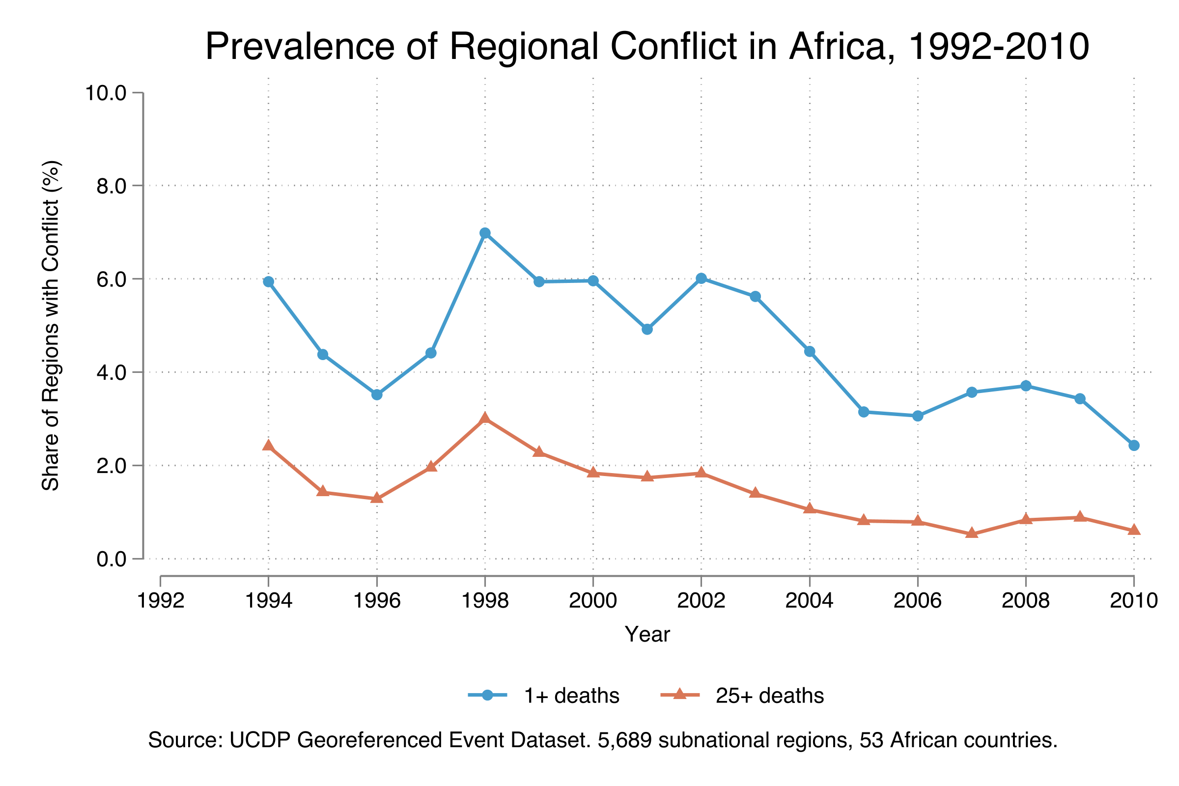
The time series of conflict prevalence shows two patterns. First, conflict with 1+ deaths (steel blue line) peaked at around 7% of regions in 1998, then gradually declined to about 2.5% by 2010. Second, severe conflicts with 25+ deaths (warm orange line) tracked a similar but lower trajectory, averaging about one-third of the any-death rate. The 1998 peak coincides with major conflicts in the Democratic Republic of Congo, Ethiopia-Eritrea, and Sierra Leone.
6. OLS with fixed effects
We begin with standard OLS panel regression as a benchmark. All regressions use the detrended variables and include year dummies, effectively controlling for region fixed effects, region-specific time trends, and year fixed effects.
xtreg ucdp_death_dummy_dt llnlight01_dt Iyear*, fe robust cluster(objectid)
Fixed-effects (within) regression               Number of obs     =     96,591
Group variable: objectid                        Number of groups  =      5,689

R-squared:
     Within  = 0.0041                                Obs per group: avg =  17.0

                            (Std. err. adjusted for 5,689 clusters in objectid)
-------------------------------------------------------------------------------
              |               Robust
ucdp_death_~t | Coefficient  std. err.      t    P>|t|     [95% conf. interval]
--------------+----------------------------------------------------------------
llnlight01_dt |   .0007773   .0011548     0.67   0.501    -.0014866    .0030411
The OLS coefficient on nighttime light intensity is 0.001 — effectively zero and far from statistical significance (p = 0.50). This near-zero result is not evidence that economic shocks have no effect on conflict. Instead, it reflects the attenuation bias from measurement error: nighttime lights are a noisy proxy for true economic activity, and classical measurement error in an explanatory variable biases the coefficient toward zero. Miguel et al. (2004) found the same pattern — their OLS estimates were also much smaller than their IV estimates — and attributed it to “the problem of measurement error in African national income figures, which are widely thought to be unreliable” (p. 727).
Reduced-form estimates
Before running the IV regressions, we check whether the instruments directly predict conflict. These “reduced-form” regressions test the numerator of the IV estimand.
xtreg ucdp_death_dummy_dt l2lnrain01_dt Iyear*, fe robust cluster(objectid)
xtreg ucdp_death_dummy_dt l2meanpdsi_dt Iyear*, fe robust cluster(objectid)
Rainfall -> Conflict:
l2lnrain01_dt |  -.0109408   .0033706    -3.25   0.001

Drought  -> Conflict:
l2meanpdsi_dt |  -.0016168   .0003894    -4.15   0.000
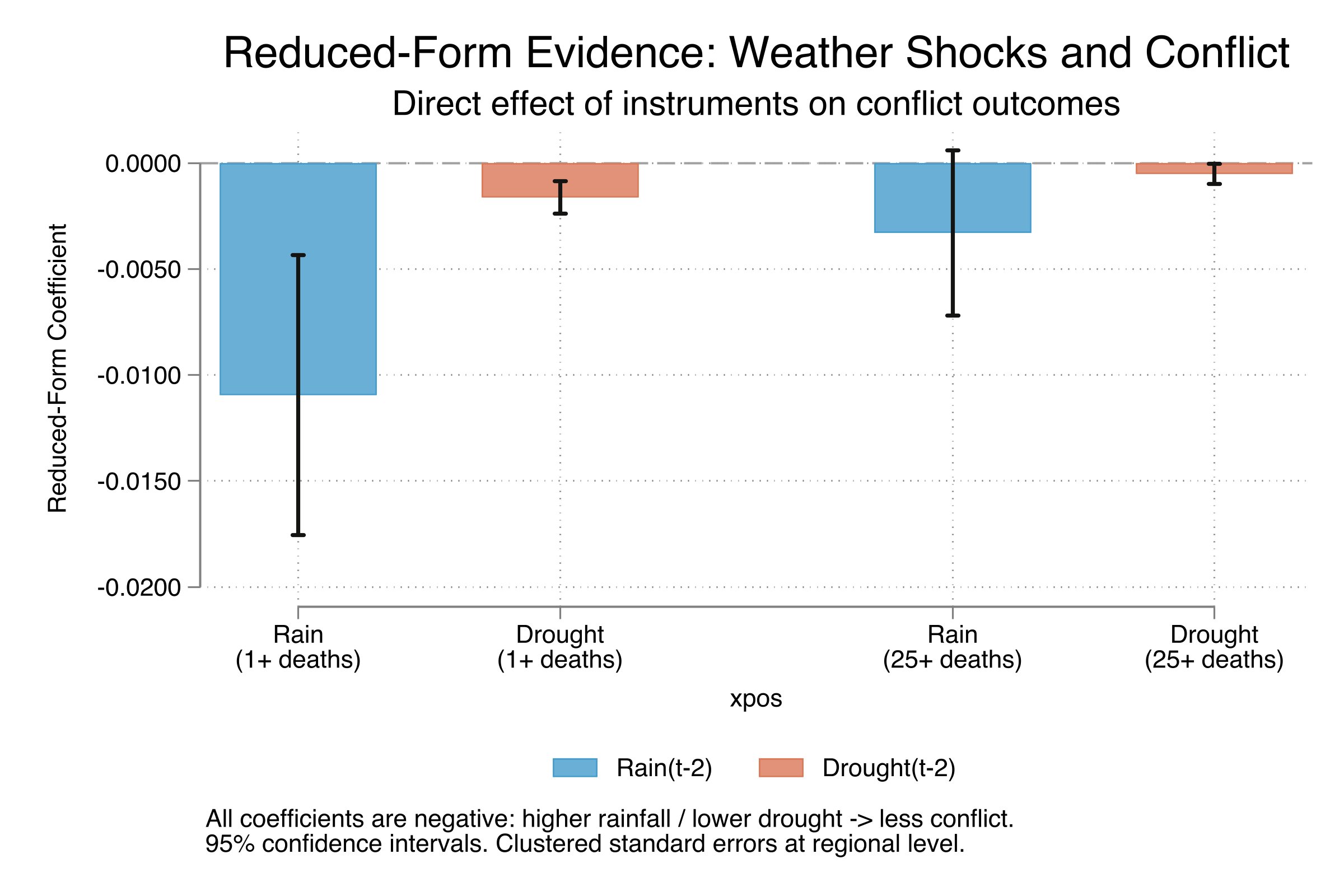
Both instruments predict conflict directly and with the expected signs. Higher rainfall (coefficient = -0.011, p = 0.001) and lower drought intensity (coefficient = -0.002, p < 0.001) are associated with fewer future conflicts. These reduced-form estimates are important: for the IV strategy to work, the instruments must not only predict the endogenous variable (first stage) but also show a relationship with the outcome (reduced form). The fact that both weather variables independently predict conflict in the expected direction is encouraging evidence for the causal mechanism: weather affects economic activity, which affects conflict.
7. 2SLS/IV estimation
Now we estimate the causal effect using two-stage least squares. The xtivreg2 command handles panel IV estimation with fixed effects, clustered standard errors, and first-stage diagnostics.
Conflict with 1+ deaths (Table 2)
// IV with Rain as instrument
xtivreg2 ucdp_death_dummy_dt (llnlight01_dt=l2lnrain01_dt) Iyear*, ///
    fe robust cluster(objectid) first

// IV with Drought as instrument
xtivreg2 ucdp_death_dummy_dt (llnlight01_dt=l2meanpdsi_dt) Iyear*, ///
    fe robust cluster(objectid) first

// IV with Both instruments
xtivreg2 ucdp_death_dummy_dt (llnlight01_dt=l2meanpdsi_dt l2lnrain01_dt) Iyear*, ///
    fe robust cluster(objectid) first
=== TABLE 2: Effects on regional conflicts (1+ deaths) ===
-------------------------------------------
                 (1)      (2)      (3)      (4)      (5)      (6)      (7)
                 OLS      OLS      OLS      OLS     2SLS     2SLS     2SLS
-------------------------------------------
Ln Lights(t-1)  0.001                              -0.303***-0.293***-0.296***
              (0.001)                              (0.111)  (0.085)  (0.076)

Ln Rain(t-2)            -0.011***          -0.007*
                        (0.003)            (0.004)

(Non) Drought                    -0.002***-0.001***
                                (0.000)  (0.000)
-------------------------------------------
Observations    96591    96591    96591    96591    96591    96591    96591
N Regions        5689     5689     5689     5689     5689     5689     5689
R-squared        0.00     0.00     0.00     0.00    -0.54    -0.51    -0.52
Instrument       None     None     None     None  Rain(t-2) Drought  Both
-------------------------------------------
Standard errors clustered at the regional level. * p<0.10, ** p<0.05, *** p<0.01
The 2SLS results are dramatically different from OLS. Using rainfall as the sole instrument (column 5), the coefficient on nighttime lights is -0.303 (SE = 0.111, p < 0.01). Using drought alone (column 6) yields -0.293 (SE = 0.085, p < 0.01), and using both instruments together (column 7) gives -0.296 (SE = 0.076, p < 0.01). The remarkable consistency across all three specifications — coefficients ranging from -0.293 to -0.303 — strongly supports the robustness of the causal finding.
The economic interpretation is striking. A negative economic shock that decreases nighttime light intensity by 10% (roughly 0.1 log points) increases the probability of conflict with at least one fatality by about 3 percentage points. Given the baseline conflict rate of 4.6%, this represents a 66% increase in conflict risk — from 4.6% to approximately 7.6% in an average region.
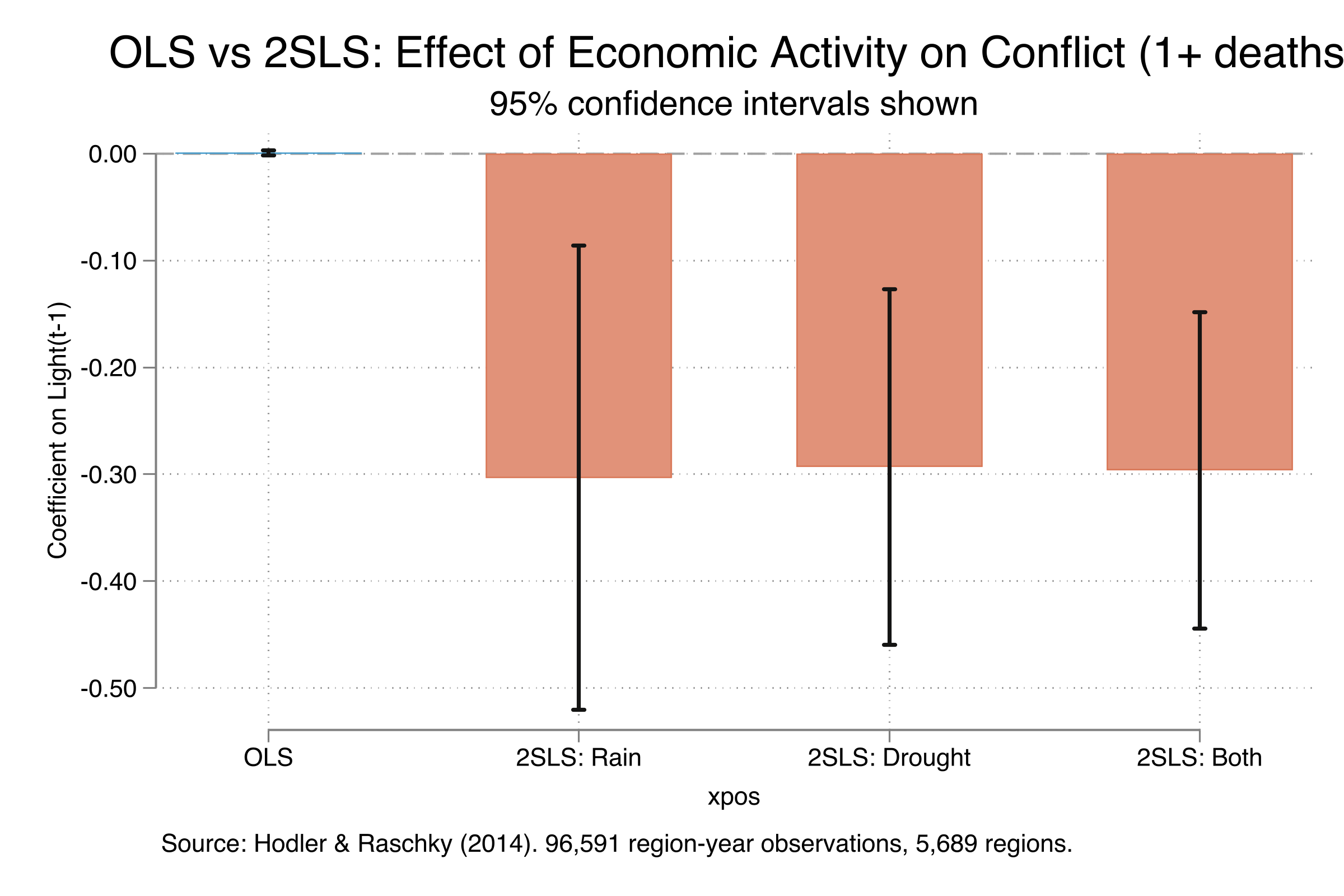
The coefficient comparison plot makes the attenuation bias visually obvious. The OLS coefficient (steel blue bar) is indistinguishable from zero, while all three 2SLS estimates (warm orange bars) are tightly clustered around -0.30 with non-overlapping confidence intervals relative to zero. The OLS-to-2SLS ratio is roughly 300:1 — consistent with severe measurement error in nighttime lights as a proxy for true economic activity.
Why is R-squared negative? The R-squared values for the 2SLS regressions are negative (around -0.52). This is normal in IV estimation and does not indicate a problem. In 2SLS, the “R-squared” is computed from structural residuals using the actual endogenous variable, not the first-stage fitted values. When the instrument-induced variation in the endogenous variable explains the outcome differently than total variation, R-squared can be negative.
Conflict with 25+ deaths (Table 3)
xtivreg2 ucdp_25death_dummy_dt (llnlight01_dt=l2meanpdsi_dt l2lnrain01_dt) Iyear*, ///
    fe robust cluster(objectid)
=== TABLE 3: Effects on regional conflicts (25+ deaths) ===
-------------------------------------------
                 (1)      (5)      (6)      (7)
                 OLS     2SLS     2SLS     2SLS
-------------------------------------------
Ln Lights(t-1)  0.001   -0.092   -0.093** -0.093**
              (0.001)  (0.057)  (0.046)  (0.040)
-------------------------------------------
Instrument       None  Rain(t-2) Drought   Both
-------------------------------------------
For severe conflicts (25+ deaths), the pattern is similar but attenuated. The 2SLS coefficient is approximately -0.09, about one-third the magnitude of the 1+ death results. A 10% decline in economic activity increases the probability of severe conflict by approximately 0.9 percentage points, which represents a 62% increase over the baseline rate of 1.4%. The drought instrument and the both-instruments specification achieve significance at the 5% level, while the rain-only instrument narrowly misses significance (p = 0.11), consistent with rainfall being a somewhat weaker instrument.
8. First-stage results and IV diagnostics
Strong instruments are essential for valid IV estimation. Weak instruments can produce biased and inconsistent 2SLS estimates, sometimes worse than OLS. We evaluate instrument strength using the first-stage F-statistic and related diagnostic tests.
xtivreg2 ucdp_death_dummy_dt (llnlight01_dt=l2lnrain01_dt) Iyear*, ///
    fe robust cluster(objectid) first
First-stage regression of llnlight01_dt:

              |               Robust
llnlight01_dt | Coefficient  std. err.      t    P>|t|
--------------+----------------------------------------
l2lnrain01_dt |   .0360693   .0072692     4.96   0.000

F test of excluded instruments:
  F(  1,  5688) =    24.62
  Prob > F      =   0.0000

Stock-Yogo weak ID test critical values:
  10% maximal IV size             16.38
  15% maximal IV size              8.96
The first-stage coefficient on rainfall is 0.036 (p < 0.001): a one-unit increase in log rainfall raises log nighttime light intensity by 0.036 units in the following year. The first-stage F-statistic is 24.62, well above the Stock-Yogo 10% critical value of 16.38. This means we can reject the hypothesis that the instrument is weak enough to cause the 2SLS size distortion to exceed 10%.
xtivreg2 ucdp_death_dummy_dt (llnlight01_dt=l2meanpdsi_dt) Iyear*, ///
    fe robust cluster(objectid) first
First-stage regression of llnlight01_dt:

              |               Robust
llnlight01_dt | Coefficient  std. err.      t    P>|t|
--------------+----------------------------------------
l2meanpdsi_dt |   .0055157   .0008685     6.35   0.000

F test of excluded instruments:
  F(  1,  5688) =    40.33
  Prob > F      =   0.0000
Drought is an even stronger instrument, with a first-stage F-statistic of 40.33 — nearly twice the strength of rainfall. The coefficient is 0.006 (p < 0.001): less drought (higher PDSI) predicts higher economic activity. This is intuitive — drought reduces agricultural output, which reduces incomes and economic activity more broadly.
Overidentification test
When we use both instruments simultaneously, the model is overidentified (two instruments for one endogenous variable). This allows us to test whether both instruments satisfy the exclusion restriction using the Hansen J test.
xtivreg2 ucdp_death_dummy_dt (llnlight01_dt=l2meanpdsi_dt l2lnrain01_dt) Iyear*, ///
    fe robust cluster(objectid) first
First-stage F-stat (Both):     25.32

Hansen J statistic:            0.007
Hansen J p-value:              0.932
The Hansen J statistic is 0.007 with a p-value of 0.932. We strongly fail to reject the null hypothesis of instrument validity. Both rainfall and drought appear to satisfy the exclusion restriction — they affect conflict only through their impact on economic activity, not directly.
Summary of IV diagnostics
| Test | Statistic | Threshold | Result |
|---|---|---|---|
| First-stage F (Rain) | 24.62 | > 16.38 | Strong |
| First-stage F (Drought) | 40.33 | > 16.38 | Strong |
| First-stage F (Both) | 25.32 | > 16.38 | Strong |
| Hansen J (overid) | 0.007 (p = 0.93) | p > 0.10 | Valid |
All three instrument specifications pass the weak instrument test, and the overidentification test supports instrument validity. These diagnostics give us confidence that the 2SLS estimates are reliable.
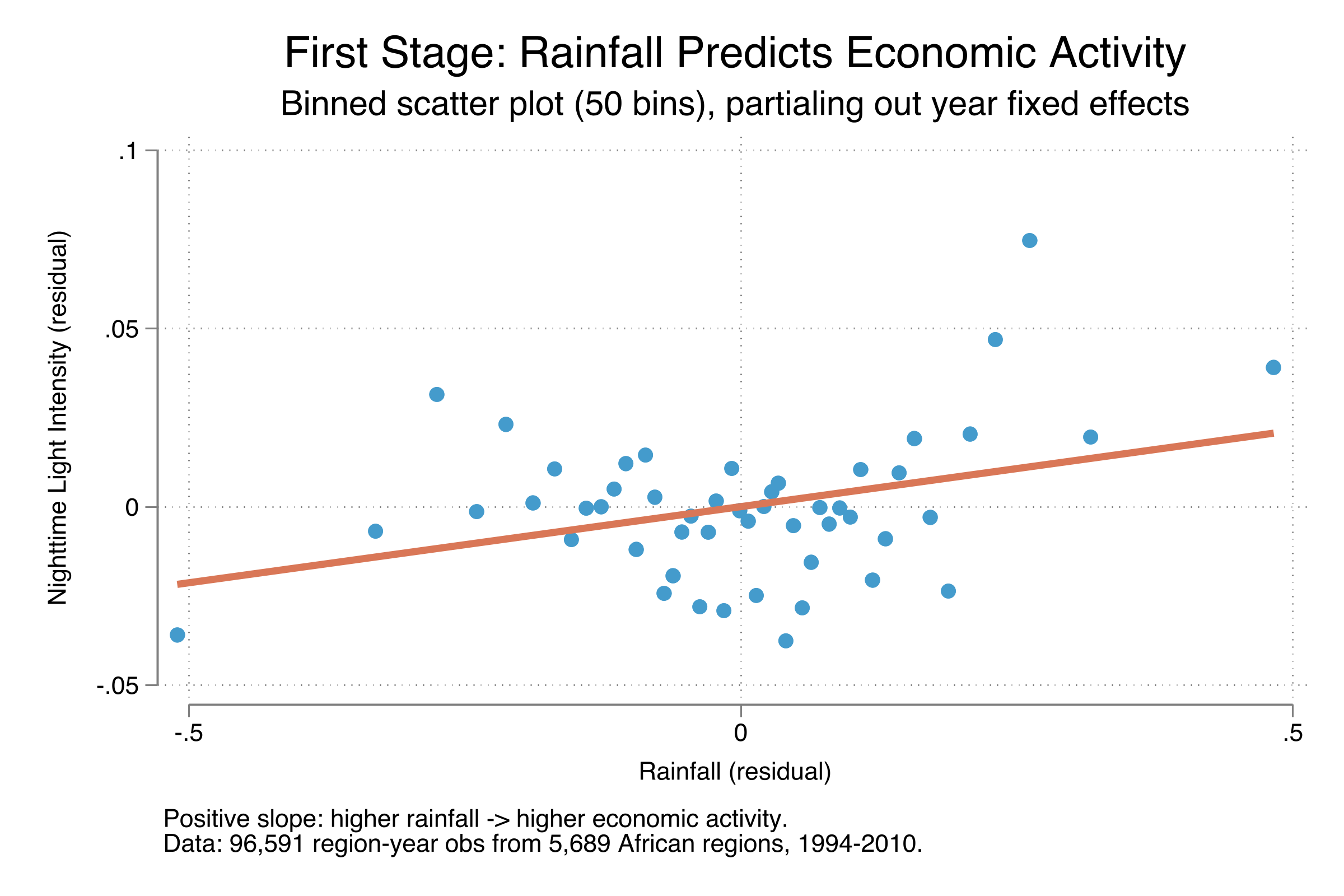
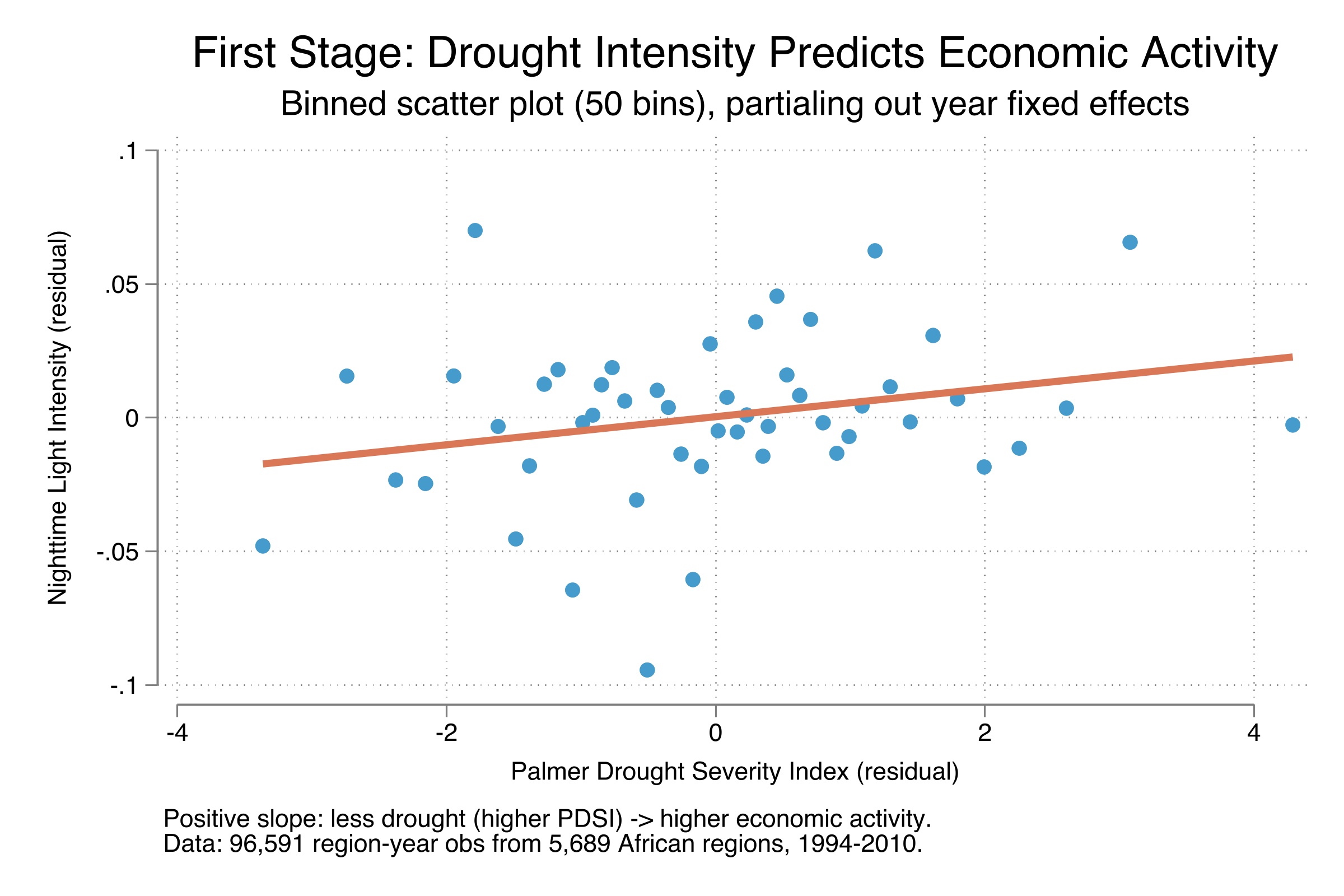
The binned scatter plots visualize the first-stage relationships. Each dot represents the average of 50 equal-sized bins after partialing out year fixed effects. Both plots show a clear positive slope: higher rainfall and less drought (higher PDSI) predict higher nighttime light intensity. The drought relationship appears somewhat tighter, consistent with the higher first-stage F-statistic (40.3 vs. 24.6).
9. Interpreting the OLS-2SLS gap
The enormous gap between OLS (0.001) and 2SLS (-0.30) estimates deserves careful discussion. Three mechanisms could explain it:
Attenuation bias (most likely). Nighttime lights are a noisy proxy for true economic activity. Classical measurement error in the explanatory variable biases OLS toward zero. The IV approach isolates the component of nightlight variation driven by weather — which is a better signal of true economic changes — effectively correcting this attenuation. Miguel et al. (2004) reached the same conclusion: “the problem of measurement error in African national income figures, which are widely thought to be unreliable” (p. 727) explains why their 2SLS estimates were also much larger than OLS.
Omitted variable bias (secondary). Unobserved factors correlated with both economic activity and conflict could bias OLS in either direction. If regions with better institutions have both higher economic activity and less conflict, the OLS estimate of the economic activity effect would be biased toward zero or even positive — consistent with what we observe.
LATE vs. ATE. The IV estimate is a Local Average Treatment Effect, reflecting the causal effect for regions whose economic activity responds to weather shocks. If these regions are more agriculturally dependent (and thus more sensitive to economic disruptions), the IV estimate could exceed the population average effect. However, most African regions are heavily agricultural, so this distinction is likely small.
10. Key takeaways
This replication confirms three important findings from Hodler and Raschky (2014):
Economic shocks cause civil conflict. A 10% decline in nighttime light intensity increases the probability of conflict with 1+ deaths by approximately 3 percentage points (from 4.6% to 7.6%) — a 66% increase in risk. For severe conflicts (25+ deaths), the increase is about 0.9 percentage points (from 1.4% to 2.3%).
OLS massively underestimates the effect. The OLS coefficient is essentially zero (0.001), while the 2SLS coefficient is approximately -0.30. This 300-fold difference is consistent with severe attenuation bias from measurement error in nighttime lights as a proxy for economic activity.
The instruments are strong and valid. First-stage F-statistics (24.6–40.3) comfortably exceed the Stock-Yogo critical value of 16.38. The Hansen J test (p = 0.93) supports the exclusion restriction. The consistency of coefficients across three different instrument specifications further strengthens the causal claim.
From a policy perspective, these results underscore that poverty reduction is conflict prevention. Programs that stabilize incomes in vulnerable regions — through crop insurance, diversification support, or social safety nets — may reduce the risk of violent conflict. The channel from weather to economic shocks to conflict also highlights the security implications of climate change, as more frequent droughts and erratic rainfall could increase conflict risk across Africa.
References
- Hodler, R. & Raschky, P.A. (2014). Economic shocks and civil conflict at the regional level. Economics Letters, 124(3), 530–533.
- Miguel, E., Satyanath, S. & Sergenti, E. (2004). Economic shocks and civil conflicts: An instrumental variables approach. Journal of Political Economy, 112(4), 725–753.
- Ciccone, A. (2011). Economic shocks and civil conflict: A comment. American Economic Journal: Applied Economics, 3(4), 215–227.
- Couttenier, M. & Soubeyran, R. (2014). Drought and civil war in sub-Saharan Africa. Economic Journal, 124(575), 201–244.
- Henderson, V.J., Storeygard, A. & Weil, D.N. (2012). Measuring economic growth from outer space. American Economic Review, 102(2), 994–1028.
- Stock, J.H. & Wright, J.H. (2000). GMM with weak identification. Econometrica, 68(5), 1055–1096.
Carlos Mendez
Associate Professor of Development Economics
My research interests focus on the integration of development economics, spatial data science, and econometrics to better understand and inform the process of sustainable development across regions.