Regression Discontinuity Design in Stata

Did a rule-based tutoring program raise exit exam scores?

+10.80parametric OLS · full sample

−8.58rdrobust LATE at the cutoff

0.58density-test p · no manipulation

Carlos Mendez

Nagoya University (GSID)

June 11, 2026

The Tension

Act I

You can’t randomize tutoring — so how do you prove it works?

A school enrolled every student scoring 70 or below on an entrance exam into free tutoring. Above 70, nothing.

The students who got help also started behind. Compare raw outcomes and you measure the program plus the gap.

The fundamental problem: students were not assigned at random. Below-cutoff students differ systematically from above-cutoff students. A naive treated-minus-untreated comparison conflates the tutoring effect with selection. The whole tutorial is about how a rule-based threshold rescues identification.

A sharp rule turns a threshold into a natural experiment

A deterministic assignment rule, drawn as a flow:

The dial

• Running variable: entrance exam score
• Cutoff: \(c = 70\)
• Score \(\le 70\) \(\rightarrow\) tutoring
• Score \(> 70\) \(\rightarrow\) no tutoring

Why it identifies

• A student at 69 vs one at 71 is nearly identical
• They differ only by which side of the line they landed
• The jump in exit scores at the cutoff is the causal effect

Students just below and just above 70 are comparable by construction — only treatment differs.

This replaces the post’s Mermaid flow diagram. The entrance exam is the running variable; the cutoff at 70 is a sharp, rule-based boundary. Comparing students immediately on either side approximates an experiment because the threshold, not the students, decides treatment.

The spoiler: a clean downward jump in exit scores at 70

Binned averages with local-linear fits each side of the cutoff. Moving left to right (tutored → not), exit scores drop ~8–10 points at 70.

This is the money chart — plant it now, earn it in Act II. Don’t explain bins or polynomials yet. Just note the visible break at 70: tutored students (left) sit above the right-side trend. The jump is downward only because we read left→right, from the tutored to the untreated group.

Where we’re going

• The lab: 1,000 students, a single 70-point cutoff
• Verify the design is sharp before estimating anything
• Estimate the LATE two ways — parametric OLS and nonparametric rdrobust
• Stress-test it: bandwidth, kernel, density, placebo cutoffs

The Investigation

Act II

The lab: 1,000 students, one threshold, 24% treated

• Running variable — entrance exam score (range 28.8–99.8, mean 78.1)
• Outcome — exit exam score (range 42.8–84.5, mean 66.2)
• Treatment — 241 students (24.1%) scoring \(\le 70\) were tutored

The entrance distribution is right-skewed — most students cleared 70, so only about a quarter received tutoring.

Five variables, 1,000 rows. We center the running variable at the cutoff (centered = entrance − 70) so the treatment coefficient reads directly as the discontinuity jump. The outcome is more compressed (SD 7.6) than the running variable (SD 12.7).

The estimand is the LATE — the jump in the CEF at the cutoff

\[\tau_{RD}=\lim_{x\downarrow c}E[Y\mid X=x]-\lim_{x\uparrow c}E[Y\mid X=x]\]

The difference between the expected exit score just above the cutoff and just below it.

Identification rests on continuity: absent tutoring, outcomes pass smoothly through 70.

Name the estimand explicitly: the Local Average Treatment Effect at the cutoff. The continuity assumption is the load-bearing one — students just below 70 would, absent treatment, look like students just above. We cannot extrapolate τ to a student scoring 30 or 95.

Before estimating, prove the gate has no leaks: 100% compliance

Position	Not tutored	Tutored	Total
Above cutoff (\(>70\))	759	0	759
At or below (\(\le 70\))	0	241	241

Zero crossovers in either direction — treatment is a deterministic function of the score. This is a sharp RDD, the strongest form.

This is the sharp-vs-fuzzy check. 100% of below-cutoff students were treated, 0% of above-cutoff. No one slipped through. A fuzzy design (say 70% take-up below, 5% above) would need an instrumental-variables-style estimator; here the discontinuity in treatment is exactly 1, so the LATE is identified directly.

See it before you estimate it: tutored students sit above the trend

Exit vs entrance scores. Blue = tutored (≤70), orange = not tutored. Dashed line marks the cutoff at 70.

Raw scatter, no smoothing. Both groups slope upward — higher entrance predicts higher exit — but the blue (tutored) cloud near the cutoff sits visibly above the orange trend extended leftward. That vertical gap at 70 is what every estimator below tries to quantify.

Parametric OLS: regress exit on the score plus a treatment dummy

\[\text{exit}_i = \beta_0 + \beta_1\,\text{entrance}_i + \tau\,\text{treat}_i + \varepsilon_i\]

The coefficient \(\tau\) is the jump at the cutoff — the treatment effect under a common linear trend.

gen centered = entrance_exam - 70
reg exit_exam entrance_exam treat, robust

The simplest specification: one slope for both sides, a level shift τ for the treated. Centering the running variable at 70 is cosmetic for this model but matters once we add interactions. Robust standard errors throughout.

Parametric OLS says tutoring adds 10.80 points

+10.80

\(\hat\tau\) on treatment, full-sample OLS (SE 0.81, 95% CI 9.22–12.38, \(p<0.001\))

10.80 points, highly significant, off all 1,000 students. The entrance-exam slope is 0.51 — each entrance point buys about half an exit point. R² = 0.27. But this imposes one linear trend on the entire score range; the next slides relax that.

More flexible specifications barely move the estimate: 9.2–10.8

Model	Specification	\(\hat\tau\)	SE	\(R^2\)
1	Linear, same slope	10.800	0.806	0.268
2	Linear, different slopes	10.797	0.816	0.268
3	Quadratic	9.223	1.198	0.271

The interaction term is essentially zero (−0.001), and R² is flat across all three — added flexibility buys nothing.

Allowing different slopes each side (Model 2) leaves τ unchanged at 10.80; the interaction is −0.001 (p = 0.98), so the entrance-exit relationship has the same slope on both sides. The quadratic nudges τ down to 9.22 with a wider SE. The story is stable — but all three impose a functional form on the whole sample. That motivates going nonparametric.

Nonparametric rdrobust: drop the functional form, keep only the locals

\[\hat\tau_{RD} = \lim_{x\downarrow c} E[Y_i\mid X_i=x] - \lim_{x\uparrow c} E[Y_i\mid X_i=x]\]

Instead of one regression through 1,000 points, fit local polynomials inside a data-driven bandwidth around the cutoff.

ssc install rdrobust, replace
rdrobust exit_exam entrance_exam, c(70)

Smaller bandwidth → less bias (more comparable units) but more variance (fewer observations). rdrobust picks the MSE-optimal \(h\) automatically.

This is Cattaneo–Idrobo–Titiunik’s local-polynomial estimator. It throws away the global functional form and only uses students within a narrow window of the cutoff, weighting by a triangular kernel. The bandwidth is the central tuning choice — and rdrobust chooses it for you to minimize mean squared error.

With an MSE-optimal bandwidth of 9.98, the LATE is −8.58

−8.58

rdrobust RD effect (robust 95% CI −12.14 to −4.54, \(p<0.001\)); only the 400 students within ±10 of the cutoff are used

The MSE-optimal bandwidth is 9.98 points, so only students scoring roughly 60–80 enter the estimate — 144 below, 256 above. The sign is negative purely by rdrobust’s left→right convention: moving rightward goes from the tutored to the untreated group, so the jump is downward. Same causal story as +10.80, smaller magnitude because it is local and assumption-light.

Same finding, two conventions — both say tutoring helps by ~9–11

Parametric OLS

• Sign: \(+10.80\)
• Sample: all 1,000 students
• Imposes a global linear trend
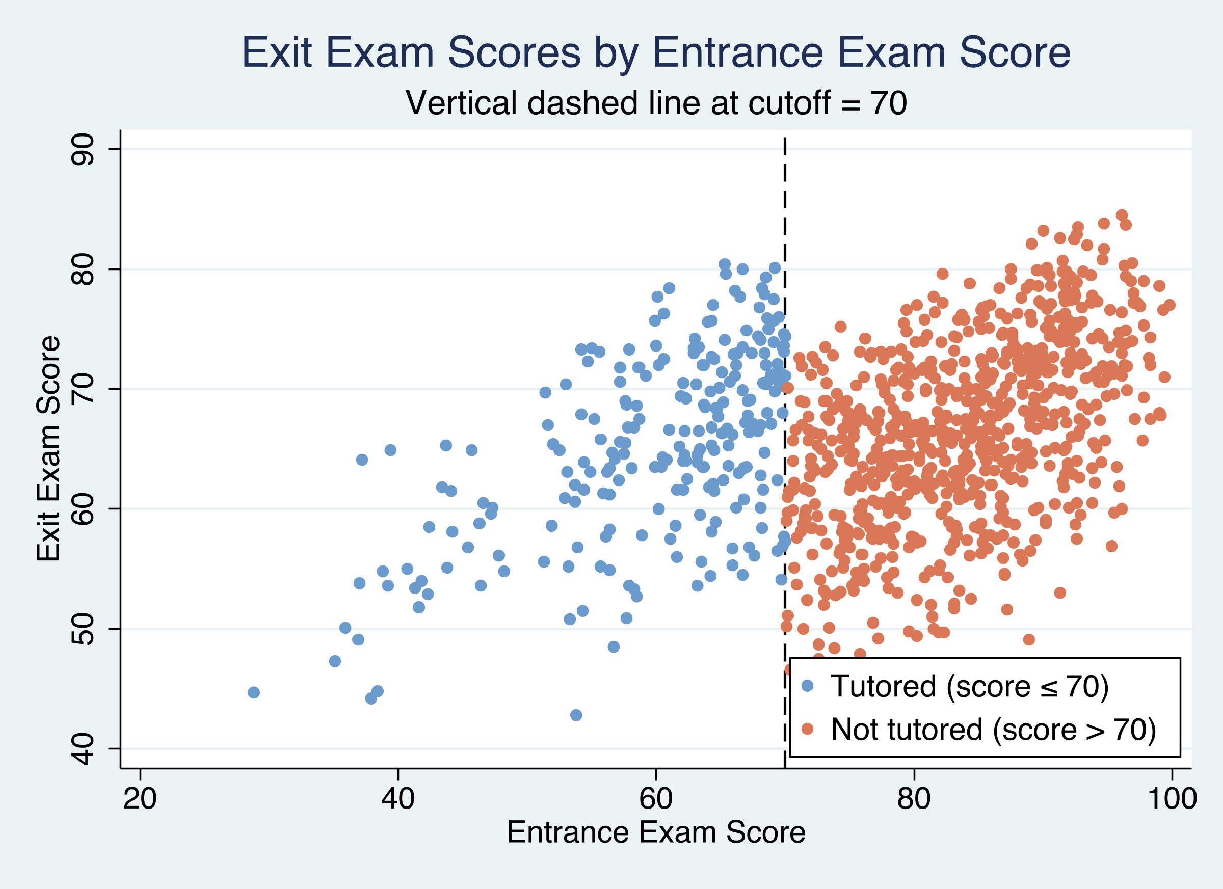
• “Effect of being tutored”

Nonparametric rdrobust

• Sign: \(-8.58\)
• Sample: ~400 near the cutoff
• No functional-form assumption
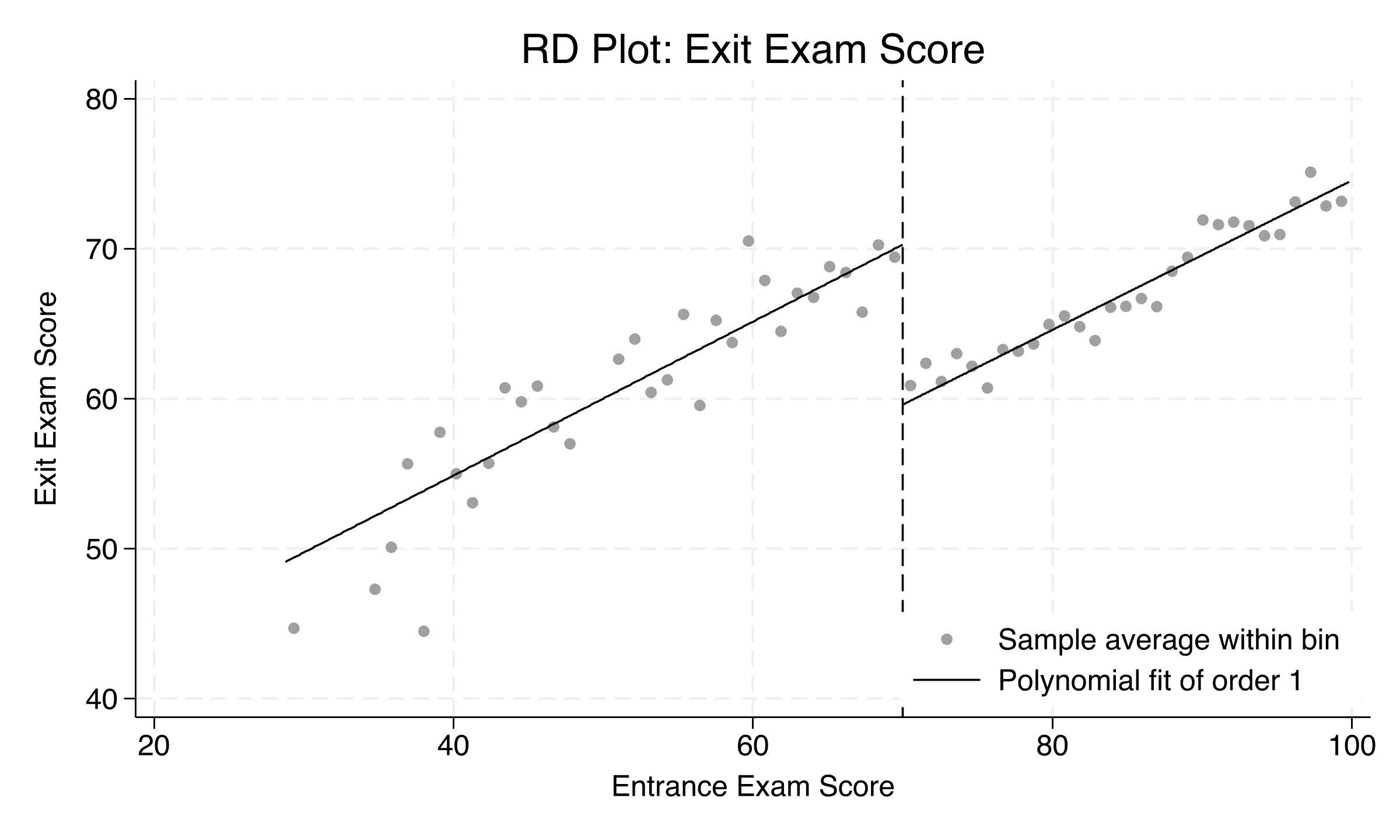
• “Jump left→right across 70”

Opposite signs, identical message: tutoring raises exit scores by roughly 9–11 points at the cutoff.

The sign flip trips up every first reader. OLS estimates the effect of treat = 1, which is positive. rdrobust estimates the discontinuity scanning left→right, which is negative because we move from tutored to untreated. They target the same LATE; the ~25% magnitude gap is scope (global vs local) plus the data-driven bandwidth.

The Resolution

Act III

The estimate barely moves from BW 5 to 20: −8.20 to −9.16

Bandwidth	\(\hat\tau\)	SE	\(p\)
5	−8.202	2.337	<0.001
10	−8.581	1.615	<0.001
15	−8.842	1.312	<0.001
20	−9.157	1.131	<0.001

Less than one point across a 4× change in window — not a bandwidth artifact.

Bandwidth is the analyst’s most discretionary RDD choice, so this is the key robustness test. From the tightest window (BW 5, a handful of students) to the widest (BW 20), τ moves less than a point and stays significant at p < 0.001. Narrower bandwidths inflate the SE (2.34 vs 1.13) as expected. The mild drift toward −9.2 hints at slight curvature far from the cutoff.

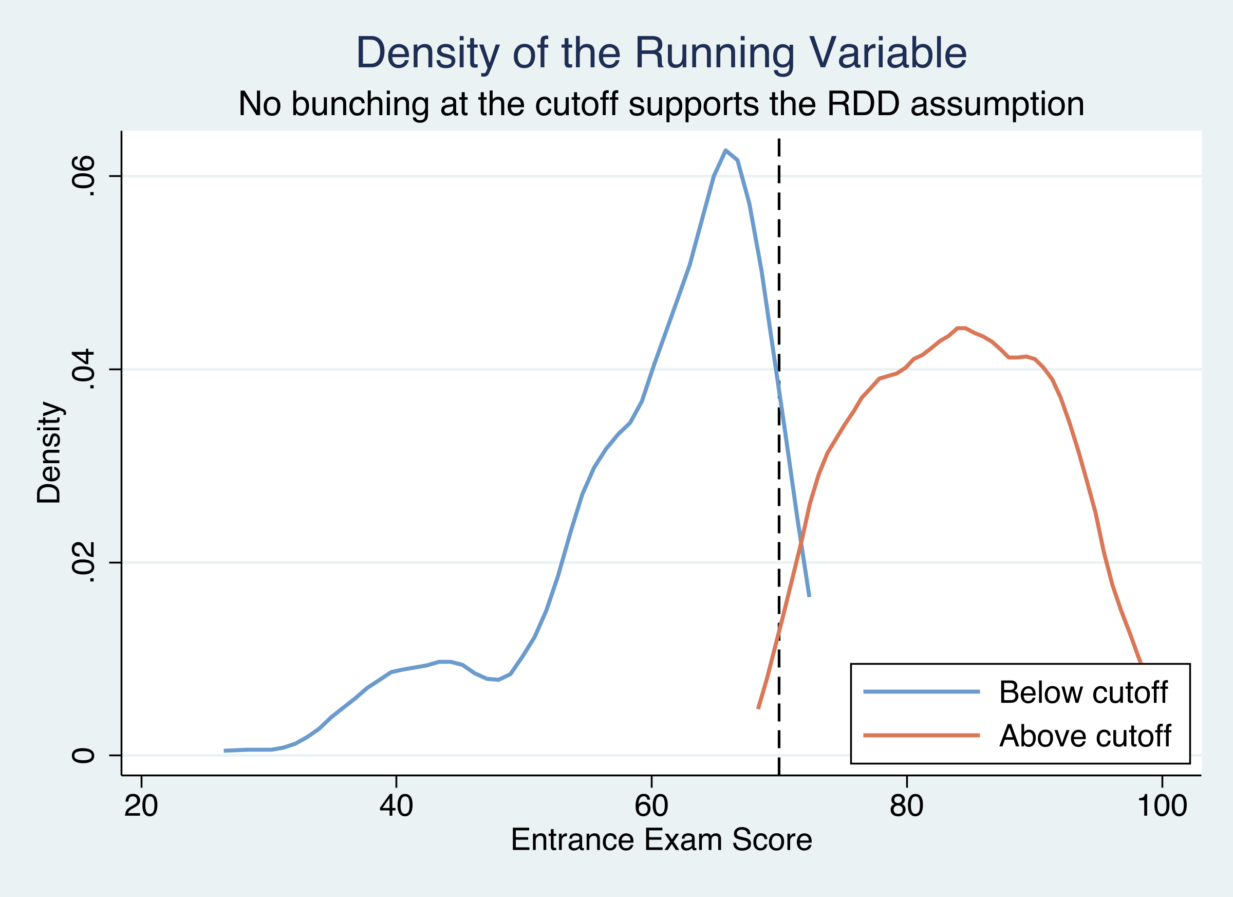
The McCrary test finds no manipulation: density p = 0.58

Kernel densities of the running variable, each side of the cutoff. Similar heights at 70 → no bunching.

RDD’s identifying assumption is that students can’t precisely sort across the cutoff. If they could game the entrance exam to land just below 70 and grab free tutoring, we’d see a spike below the line. The rddensity (Cattaneo–Jansson–Ma) test returns p = 0.58 — under a smooth density we expect a p around 0.5, so this is squarely consistent with no manipulation.

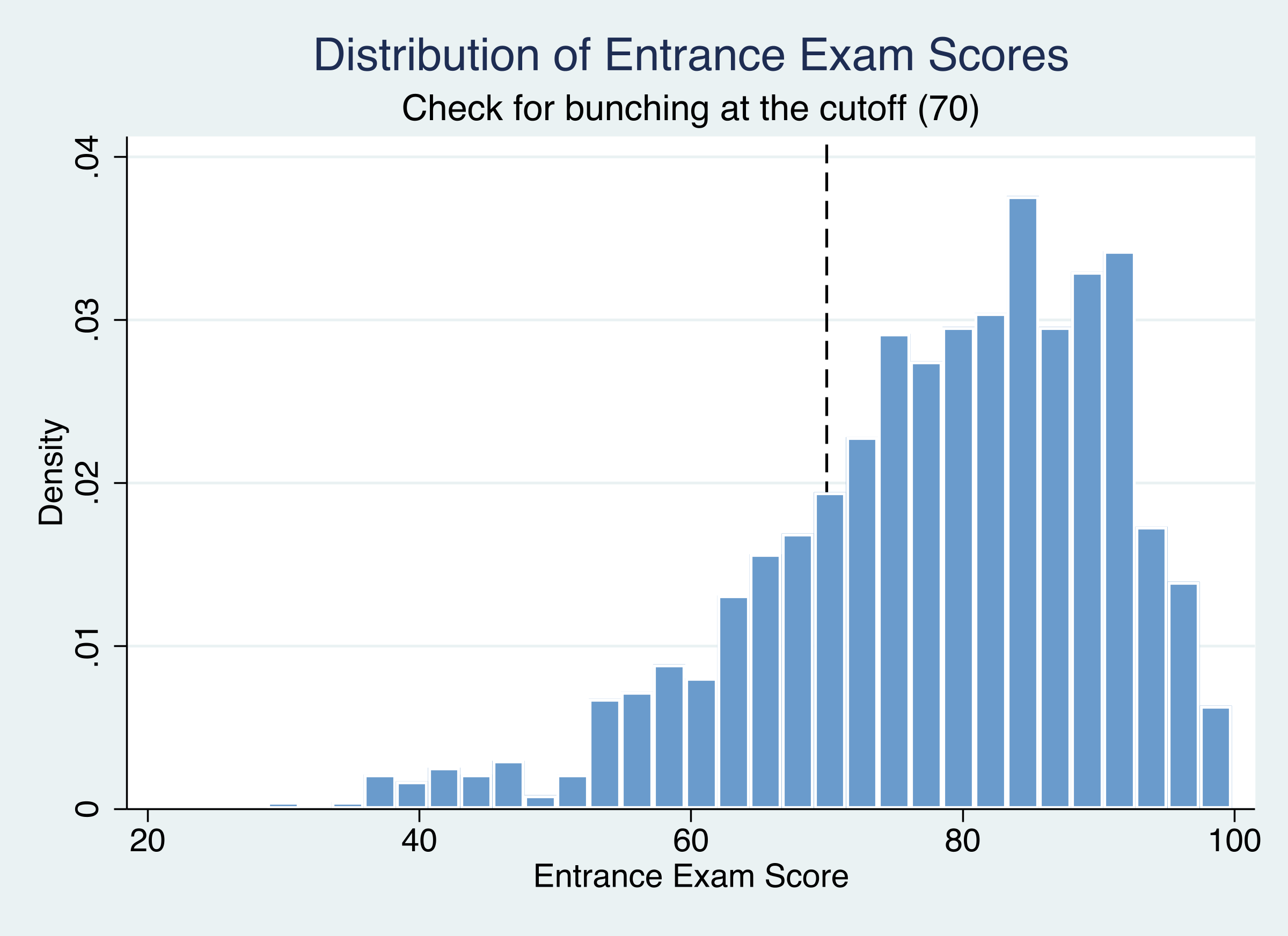
The histogram confirms it: no spike or heaping at the cutoff

Distribution of entrance exam scores; vertical line at 70. The mass transitions smoothly through the threshold.

A second, model-free look at the same question. No pile-up just below 70, no gap just above. The formal test (p = 0.58), the density plot, and this histogram all point the same way: the running variable was not manipulated. With no covariates available, these density checks carry the smoothness argument.

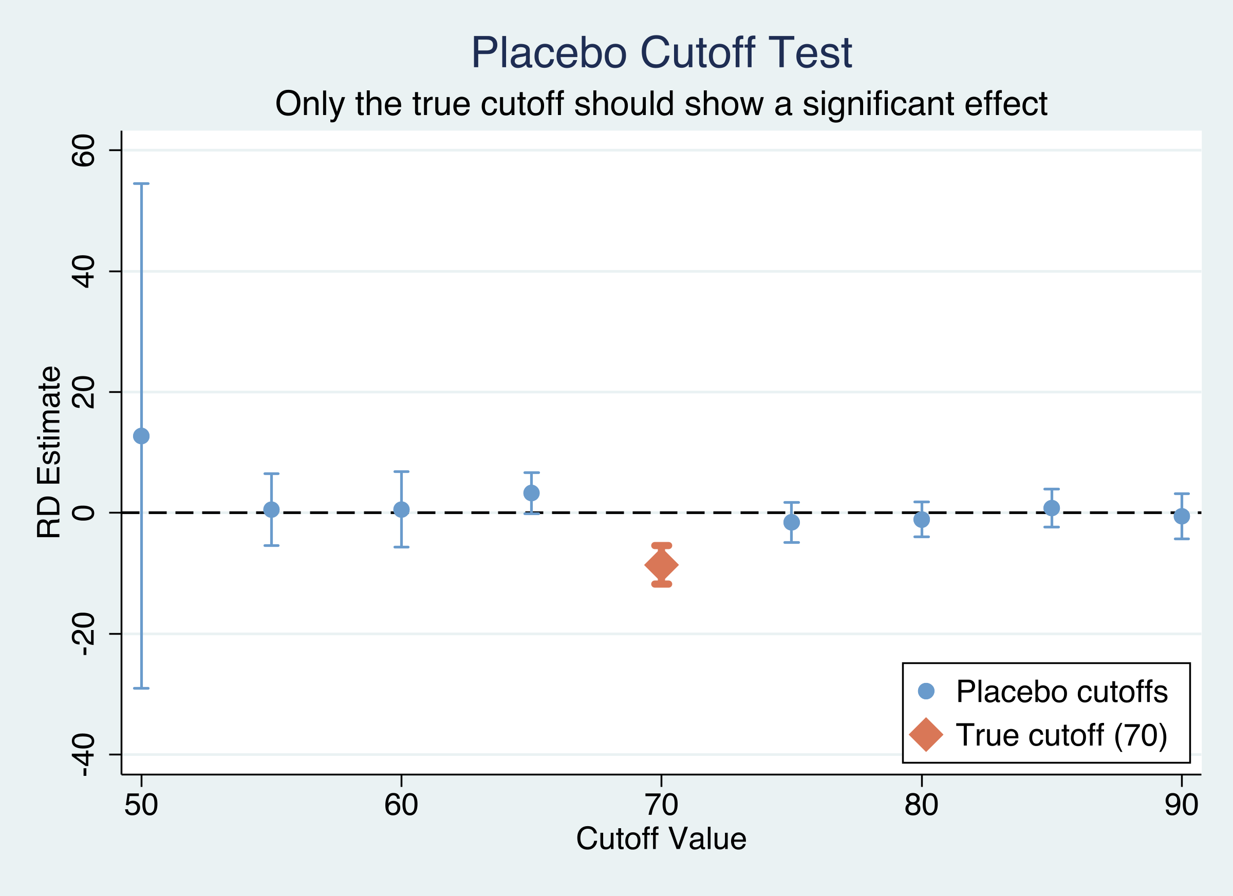
The discontinuity is unique to 70 — every placebo cutoff is null

rdrobust at 9 cutoffs with 95% CIs. Only the true cutoff at 70 (orange) excludes zero; placebos straddle zero.

If the effect were a fluke of functional form, we’d see “effects” at arbitrary cutoffs too. Testing 50, 55, …, 90, only the true cutoff at 70 is significant (p < 0.001); the eight placebos have p from 0.058 to 0.855. The borderline 65 (p = 0.058) is spillover — its ±10 window overlaps the real cutoff. This falsification test is what turns a jump into a credible causal claim.

Does machine-picking the bandwidth make this causal? No.

Objection. A data-driven bandwidth and a clever package can’t manufacture identification.

Response. Correct — and we never claim they do. Identification rests on continuity at 70; rdrobust just estimates the jump. The density and placebo tests defend that assumption — they don’t replace it.

Steelman the critique. RDD’s credibility comes from the assumption, not the estimator. We support continuity indirectly (density p = 0.58, clean placebos) but can’t prove it — and with no covariates we can’t run smoothness-on-covariates checks. The honest caveat: the estimate is local to the cutoff and says nothing about students scoring 30 or 95.

Both methods agree: rule-based tutoring lifts exit scores 9–11 points

Approach	Estimate	95% CI	\(p\)
Parametric OLS (linear)	+10.80	9.22 – 12.38	<0.001
Parametric OLS (quadratic)	+9.22	6.87 – 11.57	<0.001
Nonparametric rdrobust	8.58	4.54 – 12.14	<0.001

9–11 points is ~13–16% of the mean exit score (66.2) — passing vs failing for a borderline student.

The payoff table. Global and local methods, parametric and nonparametric, all land in a 9–11 point band, all p < 0.001. Scaled against a mean of 66.2, that’s a 13–16% gain. For policy, a sharp test-score rule is both easy to implement and easy to evaluate — but the effect remains a LATE at the cutoff.

Let the cutoff, not your model, do the identifying.

The single takeaway. When assignment follows a sharp, rule-based threshold, the discontinuity at the cutoff identifies a causal effect under continuity alone — no randomization, no functional-form heroics. Verify the design is sharp, defend continuity with density and placebo tests, and read the estimate as local. Here: tutoring adds 9–11 points at 70.