Staggered Synthetic Difference-in-Differences

Gender quotas and women in parliament — when policies arrive on different clocks

+8.03overall ATT · points · p = 0.032

−3.5 to +21.8cohort effects · real heterogeneity

9 / 7adopters · staggered cohorts

Carlos Mendez

Nagoya University (GSID)

June 11, 2026

The Tension

Act I

Most real policies don’t arrive on a single clock

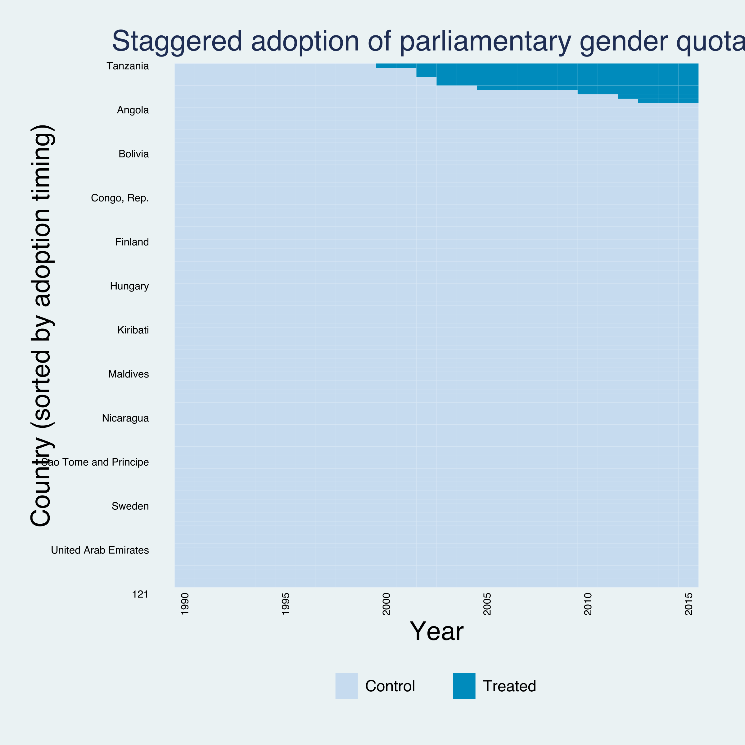
Quotas, minimum wages, carbon taxes — different units adopt in different years. Here: 9 countries adopt a parliamentary gender quota across 7 cohorts, 2000 to 2013.

The workhorse two-way fixed-effects DiD quietly breaks: it uses already-treated units as controls for later adopters. Which comparison is even valid?

This is the central tension of staggered adoption. With one adoption date TWFE is a clean DiD. With staggered timing and heterogeneous effects, the same regression becomes a variance-weighted blend of every 2×2 comparison — including “forbidden” ones where an already-treated unit serves as a control. Some of those weights are negative, so the estimate can even flip sign (Goodman-Bacon 2021; de Chaisemartin & D’Haultfœuille 2020).

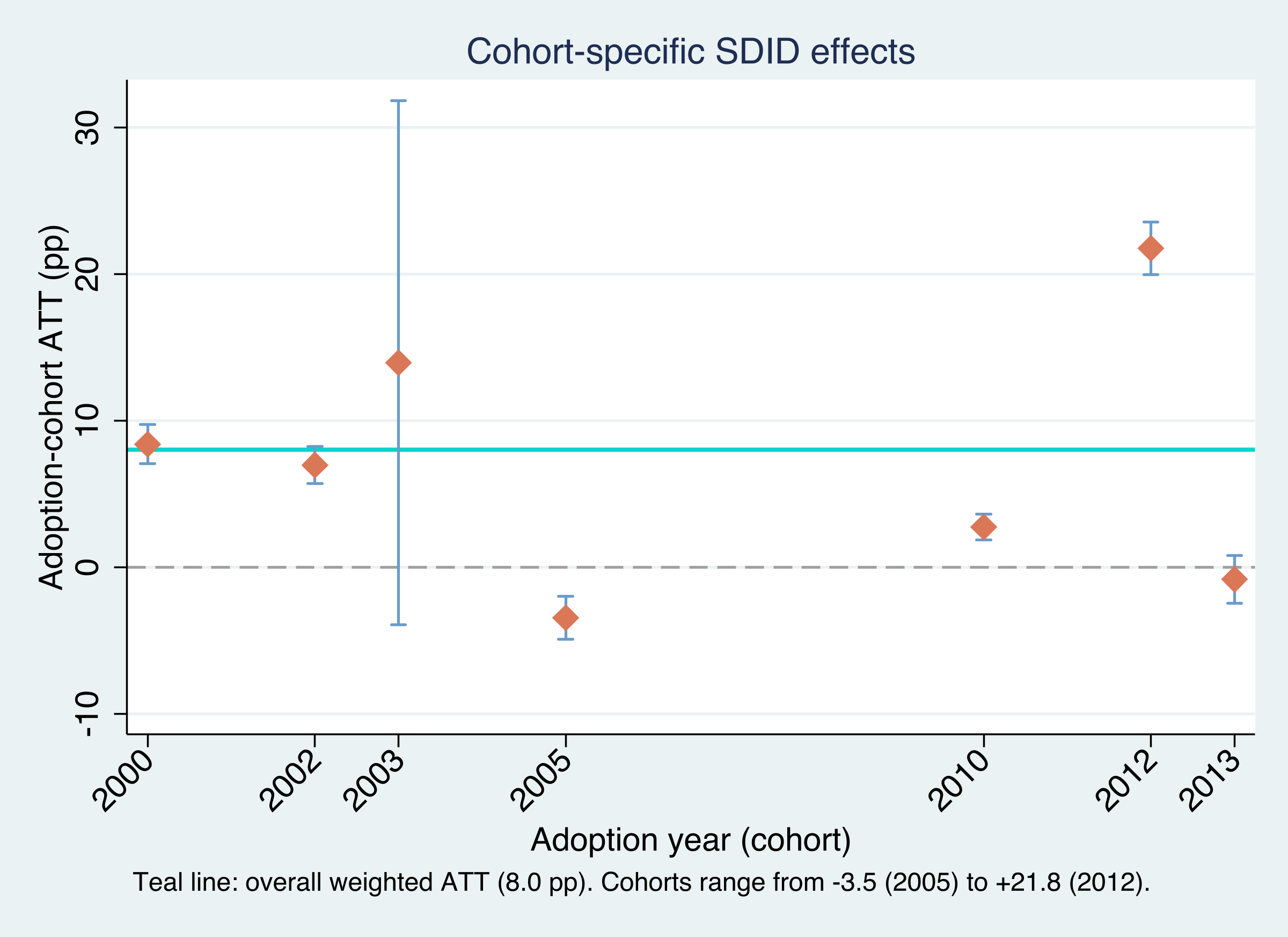
Do gender quotas raise women’s share of parliament? +8 points — but it hides a wide range

Cohort-specific SDID effects (\(\hat\tau_a \pm 95\%\) CI) with the aggregate ATT (teal). Effects swing from −3.5 to +21.8 points.

The spoiler figure. Don’t explain every cohort yet — just plant that “+8 on average” is the summary of a very heterogeneous set: the 2005 cohort is −3.5, the 2012 cohort +21.8. We earn each piece in Act II and return to this picture. The teal line is the treated-period-weighted aggregate, not the simple mean.

Where we’re going

• The data: 119 countries, 1990–2015, a staggered staircase of adoptions
• SDID from first principles — unit weights \(\omega\) and time weights \(\lambda\)
• The staggered extension — one clean SDID per cohort, then aggregate
• The event study, and three rulers for uncertainty

The Investigation

Act II

The lab: 119 countries × 26 years, 9 adopters across 7 cohorts

• Outcome \(Y_{it}\) — % of seats held by women in parliament (mean ≈ 15%)
• Treatment \(W_{it}\) — adopting a quota; absorbing (once on, stays on)
• Donor pool — the 110 never-treated countries every synthetic control is built from

Balanced panel: \(119 \times 26 = 3{,}094\) observations. Treated country-years are scarce — only 3% of the panel.

The staircase: cohorts switch on one column at a time

Treatment-timing heatmap (panelview, sorted by adoption): treated cells form a staircase in the top-right, not one shared column.

This is the visual opposite of a block design, where every treated cell would switch on in the same year-column. The staircase is the defining feature of staggered adoption — each step a cohort (2000, 2002, 2003, 2005, 2010, 2012, 2013) switching on against a sea of never-treated controls.

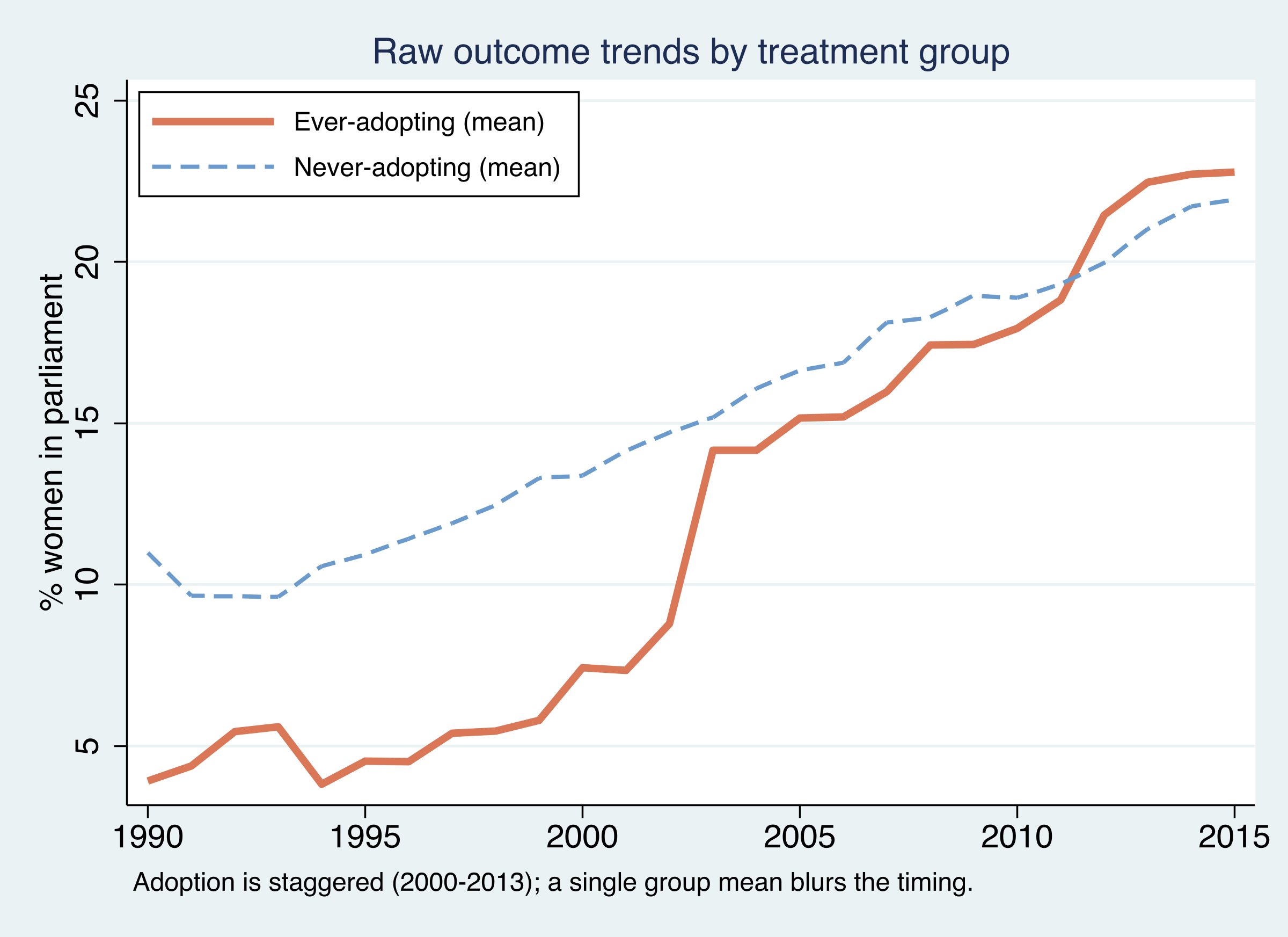
The naive two-group picture is confounded — treated start below, then overtake

Mean women-in-parliament: ever-adopting (orange) start ≈ 4% in 1990 and finish above never-adopting (blue, ≈ 22%) by 2015.

A naive eyeball DiD on these two lines would be badly confounded: the groups began at different levels, and the “treated” line aggregates countries that switched on in seven different years. This motivates the machinery — compare each cohort to a tailored synthetic control, not to the grand average.

SDID is a weighted two-way fixed-effects regression

\[\left(\hat\tau,\hat\mu,\hat\alpha,\hat\beta\right)=\arg\min_{\tau,\mu,\alpha,\beta}\sum_{i=1}^{N}\sum_{t=1}^{T}\left(Y_{it}-\mu-\alpha_i-\beta_t-W_{it}\,\tau\right)^2\,\hat\omega_i\,\hat\lambda_t\]

Run a DiD, but weight each observation by a unit weight \(\hat\omega_i\) times a time weight \(\hat\lambda_t\).

Set every weight equal and you recover ordinary DiD; the weights are what make SDID special — and each solves its own optimization.

α_i is a country fixed effect, β_t a year fixed effect, W_it the treatment dummy, τ the ATT we want. The unit and time weights are not free parameters — they each minimize their own objective, which is the next two slides.

Unit weights \(\omega\) build a synthetic control that tracks the treated trend

\[\hat\omega=\arg\min_{\omega_0,\,\omega\ge 0}\sum_{t=1}^{T_{pre}}\left(\omega_0+\sum_{i=1}^{N_{co}}\omega_i\,Y_{it}-\frac{1}{N_{tr}}\sum_{i=1}^{N_{tr}}Y_{it}\right)^2+\zeta^2\,T_{pre}\,\lVert\omega\rVert^2\]

The intercept \(\omega_0\) is the SDID twist: it lets the synthetic match the trend without matching the level — any level gap is absorbed by \(\alpha_i\). The ridge penalty \(\zeta^2\lVert\omega\rVert^2\) spreads weight across many donors.

Non-negative weights, one per donor, summing to one. Synthetic control by contrast drops the intercept and the penalty and must match the level too — that’s the difference. In the 2000 cohort, 80 donors get nonzero weight (Argentina ≈ 0.061, Guatemala ≈ 0.057), a diffuse blend rather than one or two stand-ins.

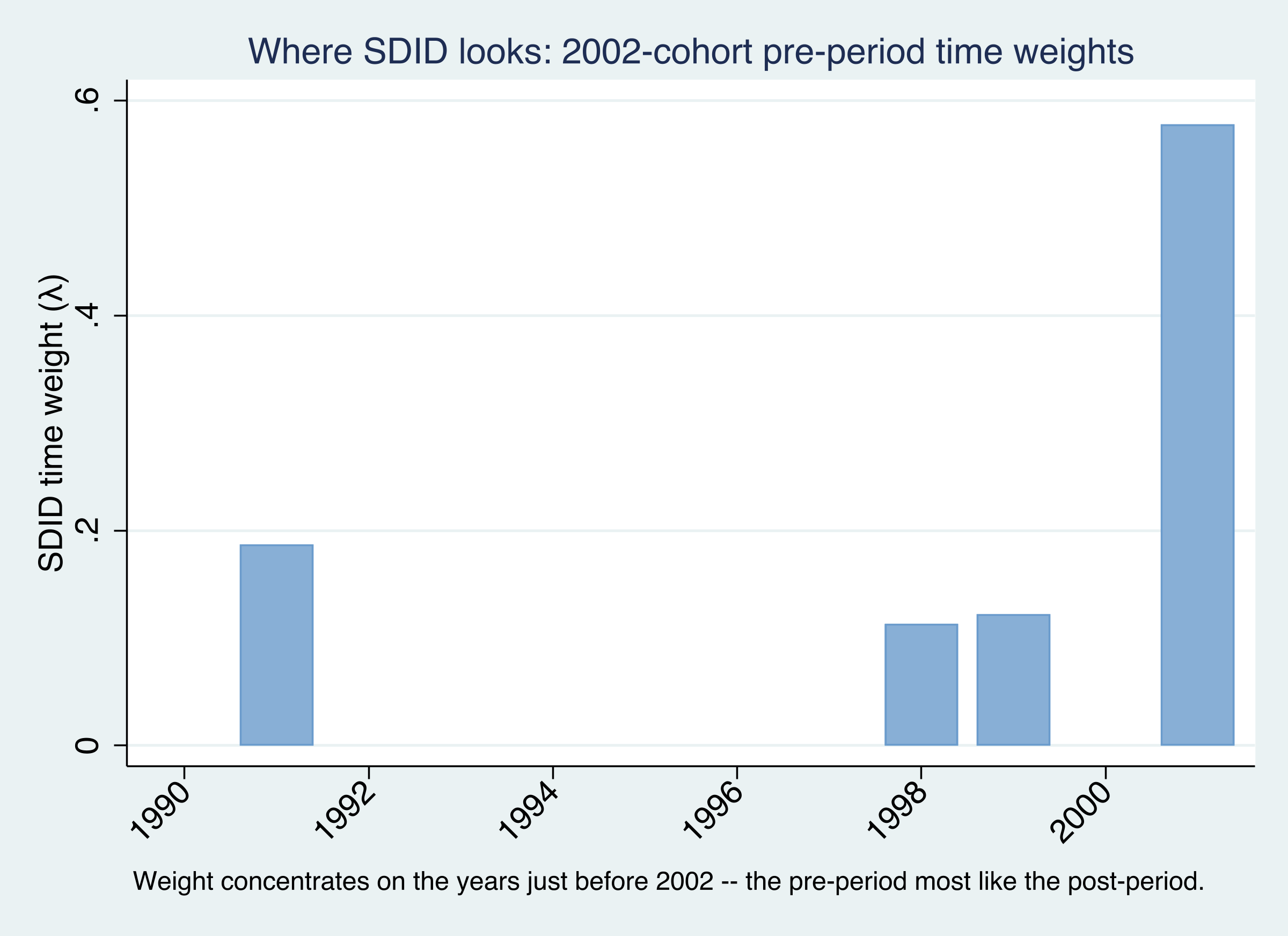
Time weights \(\lambda\) pick the “before” years most like the “after”

SDID time weights \(\hat\lambda_t\) for the 2002 cohort: weight concentrates on the late 1990s and 2001, not a flat average over 1990–2001.

The mirror image of the unit weights. Time weights choose the pre-period years that best predict each control’s post-period average, then build the baseline from the most relevant history. This is also the baseline the event study measures against — not a single “year −1.”

Three cousins, one table: SDID optimizes both weight axes

Method	Unit \(\omega\)	Time \(\lambda\)	Unit FE \(\alpha_i\)	Must match
DiD	uniform	uniform	yes	trend on all controls
Synthetic control	optimized	uniform	no	level and trend
SDID	optimized	optimized	yes	trend (level gap allowed)

Optimizing both axes — and letting the unit FE absorb the level — is what distinguishes SDID.

Staggered SDID: do the single-cohort analysis once per cohort, then average

Per cohort \(a\)

• take that cohort’s treated units + never-treated controls only
• solve SDID → its own \(\hat\omega_a,\ \hat\lambda_a,\ \hat\tau_a\)

Why it’s safe

• an already-treated unit is never a control for a later adopter
• exactly the contamination that breaks naive TWFE

Estimand: the ATT under staggered timing — the effect on the units that actually adopted, averaged over their post-adoption years.

Disarmingly simple. The block-design SDID from the previous tutorial, run once per adoption cohort. Because every cohort is compared only to the 110 never-treated countries, the forbidden comparison can never happen — that’s the whole point relative to TWFE.

The overall ATT is a non-negative, treated-period-weighted average

\[\widehat{ATT}=\sum_{a\in\mathcal{A}}\frac{N_{tr}^{a}\,T_{post}^{a}}{\sum_{b\in\mathcal{A}}N_{tr}^{b}\,T_{post}^{b}}\ \hat\tau_a\]

A cohort counts in proportion to how many treated country-years it contributes.

The 2000 cohort (treated 16 years) carries more weight than the 2013 cohort (treated 3). Unlike TWFE, every weight is positive and interpretable.

This is the staggered generalization of single-cohort SDID. When each cohort has one treated unit it reduces to the post-period share T_post^a / T_post from Clarke et al. (2024). The non-negativity is the headline contrast with TWFE, whose implicit weights can go negative.

One command runs the whole staggered procedure

sdid womparl country year quota, vce(bootstrap) seed(1213)
matrix list e(tau)          // the seven cohort effects
* covariates(lngdp, optimized) | (lngdp, projected) to condition on income

The full do-file lives in the post; these are the load-bearing lines. sdid does the per-cohort estimation and the aggregation internally; e(tau) exposes the cohort-specific effects so we can plot them. The bootstrap seed fixes reproducibility.

Compared only to never-treated controls, quotas raise women’s share: ATT = +8.03

+8.03

overall ATT (points), SE 3.74, \(t=2.15\), \(p=0.032\) · 95% CI [0.70, 15.37] excludes zero

Against a sample mean of 15% women in parliament, +8 points is a large effect and statistically distinguishable from zero at the 5% level. But this single number is the average of seven very different cohort effects — that’s the next slide.

Behind the average: cohort effects swing from −3.5 to +21.8

Cohort	\(\hat\tau_a\) (pp)	SE	Agg. weight
2000	8.39	0.68	0.170
2002	6.97	0.64	0.298
2003	13.95	9.13	0.277
2005	−3.45	0.76	0.117
2012	+21.76	0.92	0.043

The aggregate 8.03 is the weighted average; the plain mean of the seven would be ≈ 7.0.

Two of seven cohorts are negative. The 2003 cohort is essentially uninformative — SE 9.13, a CI from −4 to +32, the tell of a fragile synthetic control built from few controls. The 2000/2002/2003 cohorts carry 75% of the aggregation weight because they are early and long-exposed. (I dropped 2010 and 2013 from this table to fit the slide; full e(tau) in the post.)

One cohort up close: treated and synthetic overlap before 2002, then diverge

The 2002 treated cohort (orange) vs its anchored synthetic control (blue dashed). They track pre-2002, then split — the gap is \(\hat\tau_{2002}=6.97\).

The synthetic was built precisely to track the treated cohort before adoption. After 2002 the treated cohort climbs to ≈ 15% while the synthetic reaches only ≈ 9–10%. That post-2002 gap of about +7 points is the cohort effect, matching e(tau). Because SDID matches the trend and lets the unit FE absorb the level, we anchor the synthetic by its λ-weighted pre-period gap so the two align before adoption.

Controlling for income does not explain away the effect

Optimized (Arkhangelsky)

• adjustment folded into the SDID optimization
• ATT = 8.05, SE 3.05

Projected (Kranz)

• residualize on untreated, then SDID
• ATT = 8.06, SE 3.12

Both within 0.03 of the no-covariate 8.03 — the obvious confounder (richer countries) doesn’t account for it.

The two routes differ in how they estimate the covariate’s coefficient — optimized is flexible but heavy; projected is faster and numerically stable. They agree to the second decimal, which is reassuring. Both p < 0.01.

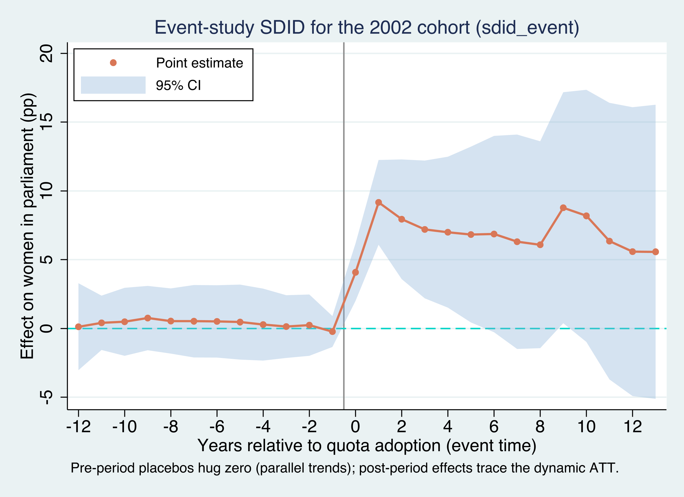
The event study: flat placebos before, an immediate and persistent rise after

sdid_event for the 2002 cohort. Left of zero = placebo (pre-trend) tests; right of zero = dynamic ATT. The baseline is \(\lambda\)-weighted, not “year −1.”

Three things to read. (1) The zero line is a λ-weighted pre-period average, not a single pre-year. (2) Left of zero are placebos — every pre-adoption coefficient sits in [−0.22, +0.76], so we can’t reject parallel synthetic trends. (3) Right of zero is the dynamic ATT: +4.1 at event time 0, ≈ +9.2 a year later, then settling +6 to +9 for over a decade. Quotas shift the level and sustain it.

The dynamic effect, in one definition

\[\delta_{\ell}=\left(\bar Y_{\ell}^{\,tr}-\bar Y_{\ell}^{\,co}\right)-\left(\bar Y_{base}^{\,tr}-\bar Y_{base}^{\,co}\right),\qquad \bar Y_{base}^{\,g}=\sum_{t=1}^{T_{pre}}\hat\lambda_t\,\bar Y_t^{\,g}\]

The treated-minus-synthetic gap at event time \(\ell\), net of the same gap at the \(\lambda\)-weighted baseline.

Pre-period \(\delta_\ell\) near zero is the parallel-trends placebo; post-period \(\delta_\ell > 0\) is the dynamic effect.

The Resolution

Act III

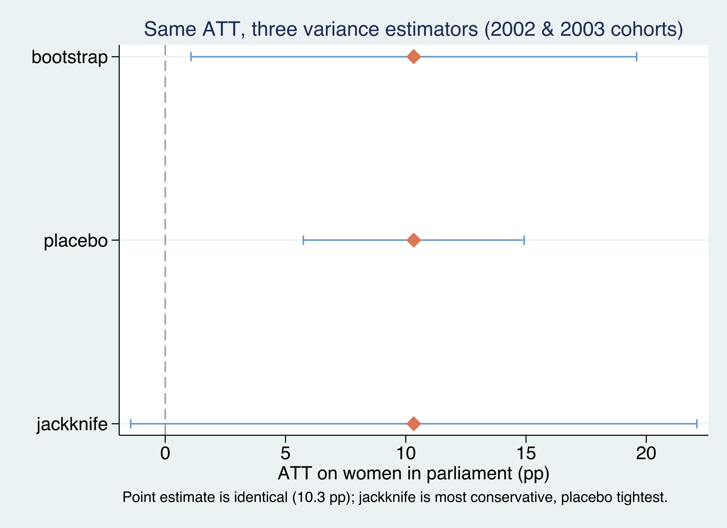
Nine treated units unlock three rulers — same estimate, different error bars

Same point estimate (10.33 on the 2002+2003 subsample), three variance estimators: jackknife widest (SE 6.01, CI crosses zero), placebo tightest (2.34), bootstrap between (4.73).

With one treated unit (California, the previous tutorial) only placebo inference was available. With nine, all three are on the table. The inference procedure changes only the SE, never the estimate. Jackknife is most conservative; placebo tightest but rests on homoskedasticity and needs more controls than treated; bootstrap is the default in between. The subsample 10.3 exceeds the full-sample 8.0 because dropping the five single-country cohorts discards the negative 2005 and 2013 effects.

Report the bootstrap — but cross-check it when treated units are few

4.7 · 6.0 · 2.3

standard errors on one ATT of 10.33 — bootstrap · jackknife · placebo. A result “significant” under placebo but not jackknife deserves caution.

The practical takeaway. The point estimate is identical to two decimals across methods; the spread differs by a factor of nearly three. With only a handful of treated units, the cautious analyst reports the widest interval. Jackknife’s CI alone crosses zero here.

Does machine-built weighting make this causal? No — assumptions still carry the weight

Objection. Choosing controls and weights from the data can’t manufacture identification.

Response. Correct. The ATT is identified only under synthetic parallel trends per cohort, no anticipation, an absorbing treatment, and no cross-country spillovers. SDID disciplines selection and weighting; it can’t rule out timing that responds to the outcome. The flat event-study placebos support parallel trends — they cannot prove it.

Steelman, don’t strawman. SDID’s contribution is non-negative, transparent cohort weighting and trend-matched counterfactuals — not a relaxation of the identifying assumptions. quota_example is a teaching subset of Bhalotra et al. (2023); these numbers illustrate the method, not a final verdict on quota policy.

A single headline number summarizes real heterogeneity — weight the cohorts transparently

−3.5 → +21.8

seven cohort effects behind one +8.03 ATT · non-negative, treated-period weighting is what makes the average honest under staggered timing

The resolution of the Act-I tension. The block design and the staggered design are two faces of one estimator — staggered SDID is just single-cohort SDID, done once per cohort and averaged with transparent, positive weights. That is the difference between an interpretable +8 and TWFE’s contaminated blend.

When policies arrive on different clocks, estimate each cohort cleanly — then weight, don’t average blindly.

The single sentence to remember. Per-cohort SDID against never-treated controls sidesteps the forbidden comparison; non-negative treated-period weights make the aggregate honest; and the event study shows the dynamics the single number conceals.