Heterogeneous treatment effects via two-stage DID

Homogeneous Treatment Effects

• 🎯 Purpose: Estimate treatment effects when the treatment is not randomly assigned.

• 📉 Parallel Trends Assumption: In the absence of treatment, the treated and untreated groups would have followed parallel paths over time.

• 🔄 Two-Way Fixed-Effects (TWFE) Model:

  • Static Model:

  $$ y_{igt} = \mu_g + \eta_t + \tau D_{gt} + \epsilon_{igt} $$

  • $ y_{igt} $: Outcome variable.
  • $ i $: Individual.
  • $ t $: Time.
  • $ g $: Group.
  • $ \mu_g $: Group fixed-effects.
  • $ \eta_t $: Time fixed-effects.
  • $ D_{gt} $: Indicator for treatment status.
  • $ \tau $: Average treatment effect on the treated (ATT).

• ❗ Limitations: Assumes constant treatment effects across groups and time, which is often unrealistic.

Heterogeneous Treatment Effects

• 🔄 Enhanced TWFE Model: $$ y_{igt} = \mu_g + \eta_t + \tau_{gt} D_{gt} + \epsilon_{igt} $$
  • Allows treatment effects ($ \tau_{gt} $) to vary by group and time.
  • Aggregates group-time average treatment effects into an overall average treatment effect ($ \tau $).

Dynamic Event-Study TWFE Model

• 🔄 Model: $$ y_{igt} = \mu_g + \eta_t + \sum_{k=-L}^{-2} \tau_k D_{gt}^k + \sum_{k=0}^{K} \tau_k D_{gt}^k + \epsilon_{igt} $$

  • Allows for treatment effects to change over time.
  • $ D_{gt}^k $: Lags and leads of treatment status.
  • Coefficients ($ \tau_k $) represent the average effect of being treated for $ k $ periods.

• 🎯 Estimation Goals:

  • Objective: Estimate the average treatment effect of being exposed for $ k $ periods.
  • Average Treatment Effect: $$ \tau_k = \sum_{g,t : t-g=k} \frac{N_{gt}}{N_k} \tau_{gt} $$
    • $ N_{gt} $: Number of observations in group $ g $ and time $ t $.
    • $ N_k $: Total number of observations with $ t - g = k $.

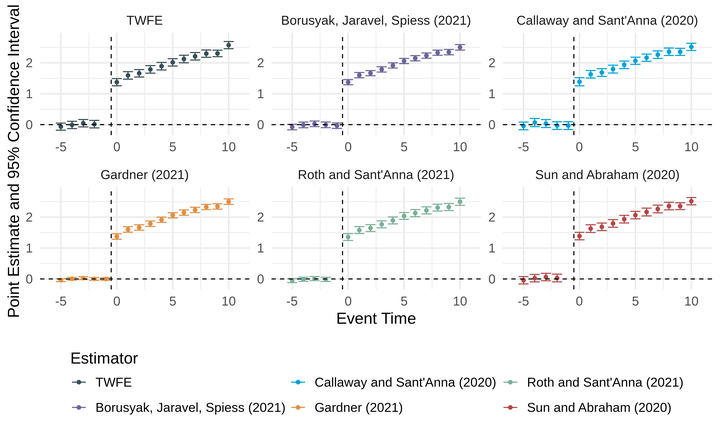
Negative Weighting Problem

• ❗ Issue: Traditional TWFE models can produce estimates with negative weights, leading to biased overall treatment effect estimates.
• 🛠 Solution by Gardner (2021):
  • Use a two-stage approach to estimate group and time fixed-effects from untreated/not-yet-treated observations and then estimate treatment effects using residualized outcomes.

Two-stage differences in differences

• 🌱 Gardner (2021) Approach:

  • 🔍 Key Insight: Under parallel trends, group and time effects are identified from the untreated/not-yet-treated observations.

  • 📜 Procedure:

    1. 🥇 First Stage:

       • Estimate the model:

         \begin{equation} y_{igt} = \mu_g + \eta_t + \epsilon_{igt} \end{equation}

       • Using only untreated/not-yet-treated observations ($D_{gt} = 0$).

       • Obtain estimates for group and time effects ($\mu_g$ and $\eta_t$).

    2. 🥈 Second Stage:

       • Regress adjusted outcomes ($y_{igt} - \mu_g - \eta_t$) on treatment status ($D_{gt}$) in the full sample to estimate treatment effects ($\tau$).

  • 🎯 Rationale:

    • The parallel trends assumption implies that residuals ($\epsilon_{igt}$) are uncorrelated with the treatment dummy, leading to a consistent estimator for the average treatment effect.